Problem: sampling complex graphs with unknown properties learned from exemplary graph sets.

Possible solution: using a state machine with transitions learned from exemplary graphs with a setup composed of node embeddings, graph embedding, categorigcal action sampling and thoroughly chosen objectives.

Note: the real underlying problems (graph embeddings or distributions of graphs) are so difficult, we are just touching the tip of the iceberg and as soon as there would be adequate approximate solutions to it, there are going to be even more fascinating applications in medicine, chemistry, biology and machine learning itself.

Introduction

Graphs are fascinating structures for study and practical applications. We use them for organizing file systems in our digital infrastructure, as well as in higher level data organization forms such as databases, e.g. for indices or other data structures. Graphs are used to represent information or search fast through it. They are also used to model chemical structures, social networks, traffic flows or even programs.

Those manifold applications led to studying graphs theoretically and empirically on various levels of abstraction. Graph theory deals with graphs as mathematical structures and properties related to them. As a research field between mathematics and computer science it also intensely deals with algorithms closely connected to graphs. Network analysis is a younger field and has arisen from social sciences and graph theory. It deals with complex networks and thus investigates on large graphs on a macroscopic level. Those graphs can very often be observed in the real world.

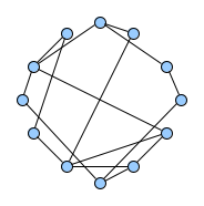
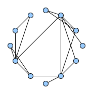
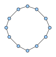
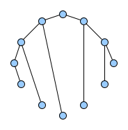
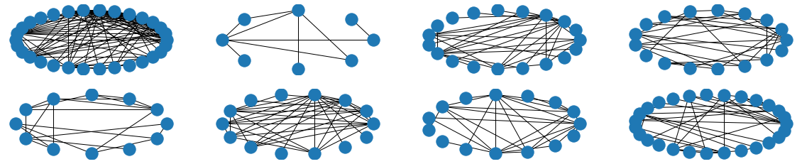
Below figures show five graphs of the same size. Based on the nature of connections between their vertices, we assign each graph a different type. Circles are an example of graphs with a constant degree of two, long shortest path lengths and simply being a circle. Trees are very well studied in graph theory and have a root and possible successors which divide the graph into branches which may not be connected amongst eachother. Vertices with no further connections than the one to their precessor are called leaves. Random graphs follow the model of Erdős-Rényi and define a large superset of graphs which have vertices connected with a distinct probability $p$. Details can be easily found online and there are actually multiple variants of an Erdős-Rényi-graph. Determining whether a certain graph is randomly connected already presents us with a statistical test. Small world graphs are to some degree random graphs and have small average shortest path lengths but higher cluster coefficients than purely random graphs as e.g. generated by an Erdős-Rényi model. Scale-free graphs are also random graphs but show a scale-free degree distribution with few vertices being connected to a very high amount of others and a lot of vertices being connected to only few other vertices.

There are many more “families” of graphs and the definition in graph theory actually allows for quite an enormous (infinite) bunch of them :)

Problem Definition

Now imagine you observe a whole bunch of graph structures. For example, we see a lot of chemical compounds for pharmaceutical usage. But we do not know what type of graph they are, we do not know the underlying process of their emergence or we simply assume that there must be some structural property hidden we do not know of and which must be somehow common among them. It could be a complex non-linear interaction of several graph theoretical properties we usually study but a visual or simple statistical analysis does not yield success.

This is the central research purpose of studying generative models of graphs. Now, could we find a generative model for sampling of the underlying, hidden distribution of graphs? This is pretty naive because, yes, we can build generative models and they even can generate graphs. But how well does such a generative model sample from the unknown underlying distribution? Answering this question and trying to answer whether two generative models are sampling from the same distribution will lead us to some statistical tests later.

Why is it even difficult to sample graphs?

First of all, graphs – or the number of possible connective structures of an increasing number of vertices – are growing highly exponential. For $n_v = |V|$ with $V$ being the set of vertices and $n_v$ being the number of vertices we have $E \subseteq V\times V$ as the set of edges. Given the number of vertices $n_v$ there are $n_g = 2^{\frac{n_v\cdot(n_v-1)}{2}}$ possible undirected graphs with no further restrictions or extensions. For $n_v = 3$ there are eight possible graphs, for $n_v = 4$ it is $n_g = 64$, for $n_v = 5$ it is $n_g = 1024$, for $n_v = 6$ it is $n_g = 32768$ and for just $n_v = 25$ vertices we would have over 2.0370e+90 possible graphs – that is more than there are probably atoms in our observable universe. Just for graphs with 25 vertices!

The number of edges for a random graph of size $n_v$ varies between zero and $\frac{n_v\cdot(n_v-1)}{2}$. However, the number of graphs of size $n_v$ having zero edges is one, the number of graphs of size $n_v$ having $\frac{n_v\cdot(n_v-1)}{2}$ edges is also one, but the number of graphs of size $n_v$ having exactly one edge is $\frac{n_v\cdot(n_v-1)}{2}$. The probability of choosing a complete graph (a graph with full connectivity) or an empty graph is significantly lower than choosing a graph with some (not zero) edges. In fact for a graph of size fifteen it is already a hundred times more likely to choose a graph with one edge than a graph with no edge.

This example shows that choosing uniformly from one property of the graph (the number of vertices) yields a highly non-uniform distribution for another property. Sampling a graph with a small set of initial parameters and a rule to “construct” the graph gives us a (random) graph generator which samples from a probability distribution over graphs. There exist several random graph generators which yield very different but distinct properties and they were already mentioned above: Erdős–Rényi, Watts-Strogatz, Barabasi-Albert. In contrast to the goal of learning generative models of graphs we refer to them as probabilistic models or random graph generators (RGG). Both, learned and analytical models for graphs could be referred as “statistical models” and we explicitly differ between learned generative models and analytical probabilistic models – analytical because we break them up into explicit rules and investigate on their emergent characteristics and learned because we try to find hidden rules or the underlying distribution for the observation of a set of graphs.

What are the use cases?

Drug Discovery / Drug Design Given drugs with certain properties such as analgetics, can we find similar drugs with some properties being the same but without having certain side-effects?

Biology / Chemistry There are various more problems in research fields such as biology and chemistry in which we could compare structures or discover new ones given sets of observations.

Structural Property Discovery Given road or rail networks, can we find structural differences between them and discover properties that favor certain behaviour? Can we find new complex systems with global distinct properties such as the above stated Watts-Strogatz or Barabasi-Albert graphs?

Dynamic Systems / Neural Architecture Search Transfering methods into a smaller space of directed (or even acyclic) graphs, can we find properties of some dynamic or chaotic systems or can we improve Neural Architecture Search by exploiting structural priors?

What are alternative techniques?

In the field of Machine Learning we identified five major approaches for generative models of graphs: First, recurrent neural networks (RNNS). They are probably the ones studied the longest as a very general and powerful statistical model (very intensive since at least the nineties and not taking the history of general statistics here into account). Secondly, variational auto-encoders (VAE) which are neural networks in which gaussian model parameters are learned and used in components called “encoder” and “decoder”. VAE are very successful in learning (approximating) unknown distributions. Thirdly, generative adversarial networks (GAN) (or a special case of artificial curiosity as Jürgen Schmidhuber would name it). GANs can be used to generate e.g. small molecular graphs or sequences in general (see Yu2017). Fourthly, reinforcement learning (RL) which follows a reward-based approach. And fifthly, something I would coin (differentiable) deep state machines (DSM). Such a technique was used by the work of [Li2018] to generate graphs and we based our analysis heavily on a model extended from this one. It is important to note at this point, that there are a lot of works mixing various aspects of those loosely named terms and some techniques are very related while others are fundamentally different. All of those techniques related to those terms can be used to learn generative models of graphs.

At this point, it is important for me to state, that I am currently highly confident, that none of these generative models always or even just sometimes capture the true hidden distribution of arbitrary graph families. Would that be the case, then we would have approximate solutions for “almost” canonical representations of graphs and we could solve a lot of very complex problems if we could solve such an NP-problem always almost certainly. We are currently investigating on making this hypothesis more clear by showing that some distributions of graphs can currently not be discriminated by state-of-the-art learned representations. However, it is still important to further investigate on generative models of graphs to understand if we can break some complexities down or if we can find approximate solutions for some cases (which the literature in recent years probably has).

What is necessary to understand Deep State Machines?

The prerequisites to understand the idea of deep state machines are not too complicated. We have a set of finite states for which we learn functions which decide given a current state to which state to transition to and this is done based on the information on the current state and a memory. This memory is integrated into the model in a differentiable manner. With the analogy of a Turing machine in mind, we simply have a finite state machine with memory. While recurrent neural networks can model this memory implicitly (they are proven to be turing-complete), deep state machines are more losely coupled independent neural networks acting on a common memory. This makes them easier to interprete because each transition-decision is basically just a draw from a multinomial distribution based on the current state and the aggregated memory. Nevertheless, the overall sequence problem of constructing a graph step by step is difficult and building up a meaningful and differentiable (continuous, but finite) memory from which a decision can be drawn is very difficult to control.

The model is trained by minimizing a cross-entropy loss for all submodules. So, we simply conduct an expectation log-loss minimization and come up with node and graph embeddings with message passing during this whole process. The learned encoder modules are used in the auto-regressive process to build a memory of the current graph state.

Common terms in the field:

• message passing with graph convolution
• logarithmic cross-entropy loss optimization with stochastic gradient descent and backpropagation

Graph Construction Sequences

Why construction sequences?

How would you feed a graph into a simple discriminative model (e.g. a logistic regression binary classifier) to let it decide whether the given graph is a circle or a tree or a scale-free network? In image classification, we have canonical two-dimensional real-valued (3-colored) representations which are highly sufficient to discriminate between a car and a dog (see for the cifar10 or imagenet challenges). For graphs, we have different representations of which the adjacency list, the adjacency matrix and the incidence matrix are the most popular and well-studied ones. However, those representations are not canonical and if there would be an easy canonical representation we would have a clear solution for the graph-isomorphism problem which computational complexity is not finally resolved up to date.

To get back to the original question, the idea of a construction sequence is to represent a graph as a sequence of basic operations, mostly adding a vertex or an edge. That doesn’t solve the problem of a canonical representation but it poses the learning problem in an interesting approachable way. This construction representation poses the problem of learning “the right” sequence to come up with a certain type of graph as an auto-regressive problem as used by Yu2017 and Li2018. The advantage in case of the here presented deep state machine approach is, that the decision for a graph of any size whether to add another vertex or edge can be more easily analysed as we have separate modules which decide on exactly that.

Examples:

• The null or empty graph is represented by the empty sequence [ ].
• Graph with a single vertex is denoted with [ N ]
• Graph with two vertices connected to eachother is denoted with [ N N E 0 1 ]
• For a directed graph with two edges between two nodes the sequence extends to [ N N E 0 1 E 1 0 ]

Variants to obtain construction sequences

While the idea of having a constructive (or “evolutionary”) approach to a family of graphs, it might happen that we do not know or can not observe the single steps in which graphs are constructed. Otherwise we ourselves as humans could reason on the constructive process of the graph structures. And that is what actually often happens, e.g. in chemistry where we know rules of how atoms and molecules form higher level structures. Also, in cases of above mentioned probabilistic models, we actually know of the constructive process of e.g. scale-free networks and can use this circumstance to generate “true sequences” of such graphs. For other empirical sets of graphs, however, we need another way of coming up with a construction sequence for each contained graph. We demonstrated that by the two common graph-traversal algorithms “breadth-first-search” and “depth-first-search” and show in visualizations of our experiments that it makes a significant difference for the learning model with which traversal method it learns the graphs.

Deep Graph Generators

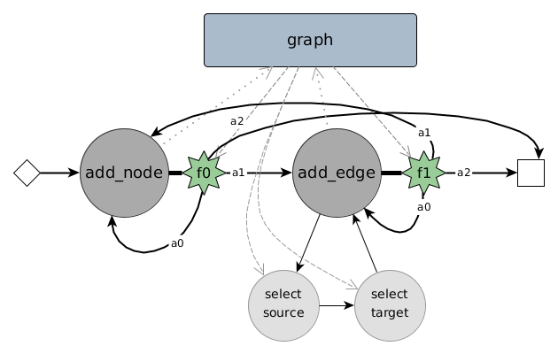
To learn a certain hidden distribution of graphs and then generate new graphs from it, we use a combination of a state machine, learnable modules (neural networks) and embedding techniques for graph elements. As depicted in above figure, the state machine consists of two major states: adding a node and adding an edge. After performing the particular task of a state a decision has to be made: transitioning from the current state to itself, to another state or to a halting / end state. For the state add_node we particularly learn a function over a multinomial distribution deciding on one of three possible transitions: $a_0, a_1, a_2$ (denoting actions). This decision is made based on a selected part of the memory, which simply consists of a graph embedding, an aggregated form of multiple node embeddings.

Whether this graph embedding reflects some useful information about the graph and its current constructive state highly decides on the ability of the whole generative model to represent the hidden distribution of graphs. We argue, that most likely up to today there are no learnable graph embedding techniques which are sufficient in deciding on a structural change to gear the whole constructive graph towards a certain structural family, but we can neither prove nor disprove this empirically with our current setup and also do not know of any sufficient empirical evidence. Technically and theoretically the learned embedding could come up with a representation sufficient to decide on the next step or action to take within the state machine.

How is the embedding learned? First of all, there are multiple types of embeddings: for vertices, for edges and an aggregated one for representing the whole graph. Node embedding techniques are already quite complex to evaluate and understand. In this work, we used Graph Convolutions from Kipf2016 which nowadays fits nicely into the message passing framework in implementations such as DeepGraphLibrary or StellarGraph. We initially set the graph embedding for an empty graph in memory of the state machine to a zero vector $h_v = (0,\dots,0)$ which has the dimensional size of $H_g = 2\cdot H_v$ with $H_v = H_e = 16$ being the dimensions for vertex and edge embeddings. The graph embedding is further obtained through a reduction, a graph convolution and an aggregation step. Namely those are $f_{reduc}, f_{conv}$ and a common mean aggregation (e.g. *torch.mean*):

$$ f_{reduc}: \mathbb{R}^{H_v}\rightarrow\mathbb{R}^{H_r}, \boldsymbol{h}_v \mapsto \sigma\left( W_{reduc}\cdot\boldsymbol{h}_v + b_{reduc} \right) $$

$$ f_{conv}: \mathbb{R}^{n_v\times d_{in}} \rightarrow \mathbb{R}^{n_v\times d_{out}}, f_{conv}(H^{(l)}, A) = \sigma\left( D^{-\frac{1}{2}} \hat{A} D^{-\frac{1}{2}} H^{(l)}W^{(l)} \right) $$

For the graph convolution $f_{conv}$ of Kipf2016 we simply choose the input dimension to be the reduced vertex representation $H_r$ and by setting $d_{out} = H_g$ we obtain a graph embedding as aggregation through $mean: \mathbb{R}^{n_v\times H_g}\rightarrow\mathbb{R}^{H_g}$ and we chose to use the mean as we observed that it was more stable with respect to exploding losses and exploding embedding values compared to e.g. the sum.

Over time of the training process we further learn initialization functions which derive vertex and edge embeddings from the current graph embedding: $$ f_{init,v}: \mathbb{R}^{H_g} \rightarrow \mathbb{R}^{H_v} $$ While the graph embedding $\boldsymbol{h}_g$ will be initialized as a zero vector at the beginning, the model (hopefully) learns to come up with meaningful initializations for a vertex embedding $\boldsymbol{h}_v$ or an edge embedding $\boldsymbol{h}_e$ (respectively with $f_{init,e}: \mathbb{R}^{H_g} \rightarrow \mathbb{R}^{H_e}$).

All of those functions are integrated in the overall end-to-end model and learned indirectly through joint log-loss-optimization of the below following decision functions. Thus, DeepGG is an example of a more complex composition of multiple modules and while we observe a growing number of such complex models we also note that they are getting more and more decoupled and interchangable, which will hopefully lead to a world in which we will share learnable modules to compose larger slightly intelligent systems.

Deep State Decisions for a state in the above sketch of DeepGG a decision has to be made for which transition to take. Those are actually transition decision functions, being own neural networks (or non-linear, restricted computational graphs) on their own. For a state index $\kappa\in\mathbb{N}$ we have a state $s_{\kappa}$ and a decision function $f_{s_{\kappa}}:\mathbb{R}^{H_{s_{\kappa}}}\rightarrow\{1,\dots,n_{s_{\kappa}}\}$. The decision is derived from the current graph embedding and additional context information, e.g. a single vertex or edge embedding. Thus $H_{s_{\kappa}}$ is for example a concatenation of multiple embeddings from the current memory of the state machine and can be $H_{s_{\kappa}} = H_g$ or $H_{s_{\kappa}} = H_g + H_v$ depending on the particular state. Given this decision and an exemplary construction sequence with single state transitions, we can compute the cross entropy loss of the decision. This decision is depicted in above figure of *DeepGG* as one of the possible actions $a_0, a_1$ or $a_2$ and over hundreds of such decisions a loss can be accumulated.

A particular difficult aspect of the model is to choose source and target vertices for constructing a new edge. Those are sub-states of the state add_edge and consist of a module $f_{c_{\delta}}$ coming up with a single vertex number. This module is a core trick of the overall model (also in DGMG) but also contains the criticial issue of why it most likely behaves strongly like a graph generator of scale-free networks. The module needs to come up with a choice from a growing multinomial distribution based on the current graph embedding and some possible context embeddings (the current memory). However, this choice is most likely to produce high and erratic loss values because it is often not easy to determine if a very particular vertex needs to be chosen as source or target. Details of how it works can be found in the article, see Stier2020.

The overall training objective is simply the joint log-loss of state decision modules and the source/target vertex choice module. Stochastic gradient descent with a learning rate of $\eta = 0.0001$ is chosen and there are also some other hyperparameters for the message passing rounds in learning the graph embeddings. Backpropagation is used to adapt the parameters of the whole end-to-end model over thousands of construction sequences.

Visual and Experimental Results

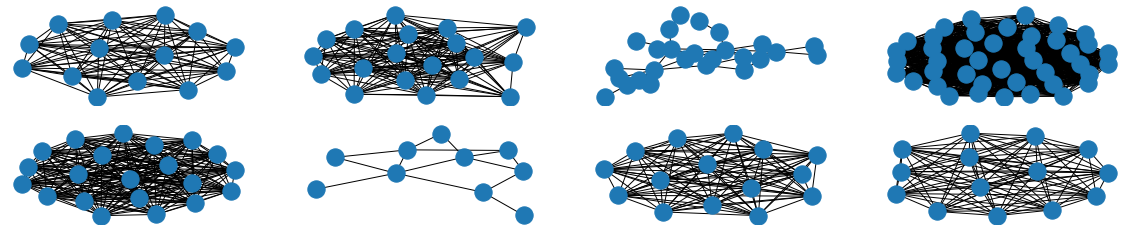
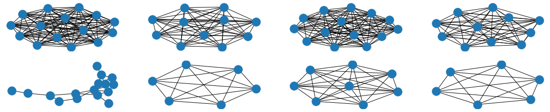
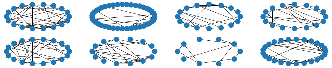
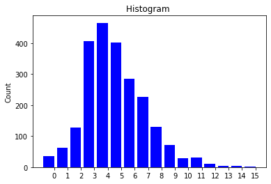
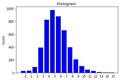
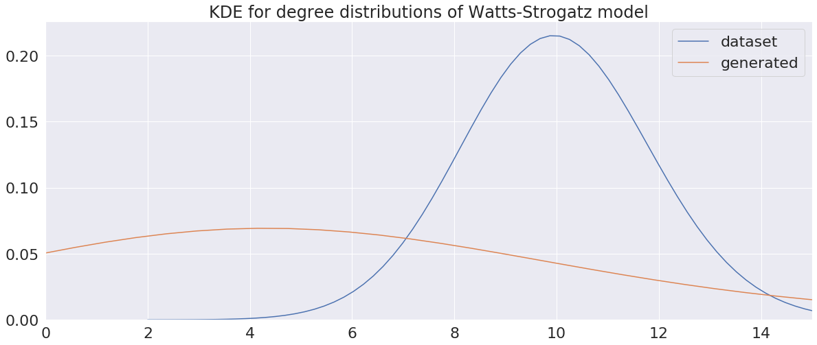
The visual results are quite interesting and show that the setup basically works - however, we find strong evidence, that especially DGMG must have a strong bias towards generating scale-free (BA-graphs) and also DeepGG most of the time does not resemble simple global properties of the underlying graph family. For example, the degree distribution of examples from an Erdos-Renyi dataset is often quite close to the one of BA-graphs, meaning that there is evidence for a skewed distribution. And this goes along with the idea of simply assigning a random sampling function to transition functions of our state machine: if the transitions are chosen randomly, we resemble a very similar behaviour as iteratively building a Barabasi-Albert graph.

Advantes and Disadvantages of this model

Pro: The design of the state machine with submodules makes it possible to understand iterative design choices of the generative model. Furthermore the design still allows an end-to-end optimization process with log-loss-minimization which needs no further supervision.

Contra: The computation times for multiple modules and especially the propagation rounds and graph convolutions are pretty expensive. This results in current computational limits for graphs of larger than 150 vertices. We only know of few works (e.g. GRAN) that report on generative models of larger graphs. However, we currently follow the assumption that those models are not sufficiently tested with statistical tests to accertain whether we can really learn hidden distributions of graphs.

Future Work

We follow several paths in improving generative models on graphs and try to transfer some of them into new areas such as Neural Architecture Search or molecular drug design. Research questions currently comprise:

• can graphs with global known properties be discriminated by selected state-of-the-art embedding techniques?
• can we use generative adversarial networks for graph generation given that we have a working discriminative model?
• can we formulate a generative model for empirical graph distributions in an evolutionary approach by exploiting facts from graph theory?
• can we enhance analyses in neural architecture search studies based on graph properties?

Thanks for being interested in our work!

See for some references below :)

References

1. Structural Analysis of Sparse Neural Networks

@article{stier2019structural,
  title={Structural Analysis of Sparse Neural Networks},
  author={Stier, Julian and Granitzer, Michael},
  journal={Procedia Computer Science},
  volume={159},
  pages={107--116},
  year={2019},
  publisher={Elsevier}
}

2. Deep Graph Generators

@article{stier2020deep,
  title={Deep Graph Generators},
  author={Stier, Julian and Granitzer, Michael},
  journal={arXiv preprint arXiv:2006.04159},
  year={2020}
}

3. Learning deep generative models of graphs

@article{li2018learning,
  title={Learning deep generative models of graphs},
  author={Li, Yujia and Vinyals, Oriol and Dyer, Chris and Pascanu, Razvan and Battaglia, Peter},
  journal={arXiv preprint arXiv:1803.03324},
  year={2018}
}

4. Seqgan: Sequence generative adversarial nets with policy gradient

@inproceedings{yu2017seqgan,
  title={Seqgan: Sequence generative adversarial nets with policy gradient},
  author={Yu, Lantao and Zhang, Weinan and Wang, Jun and Yu, Yong},
  booktitle={Thirty-First AAAI Conference on Artificial Intelligence},
  year={2017}
}

5. Semi-supervised classification with graph convolutional networks

@article{kipf2016semi,
  title={Semi-supervised classification with graph convolutional networks},
  author={Kipf, Thomas N and Welling, Max},
  journal={arXiv preprint arXiv:1609.02907},
  year={2016}
}