The following is a summary of technical thoughts and discussions within a large bi-lateral research project called Human+. An ethical board and social & legal research accompanied our technical investigations on the topic and we have always been in active and substantial exchange with involved aid organizations such as the Bavarian Red Cross, the Johanniter Order or the Federal Agency for Technical Relief THW. You can read on german articles at the german BMBF, at the Fraunhofer IAIS or at Kiras.
During the Human+ research project, we had the opportunity to investigate on migration related research. Our part of the research group was twofold:
- we investigated on possibilities to leverage Social Media information as a way to support aid organizations in their decision making in a moment of migration crisis
- we investigated on forecasting and simulation techniques given migration numbers on different temporal or geographical resolutions
In this summary, I’ll stick to the second part of forecasting&simulation, describing some ideas we experimented on. Basis of our research have been migration data of the UNHCR, which provides a pretty good temporal resolution on a daily basis for several countries on the Balkan route for the migration crisis in 2015.
The intention of this text was mainly to summarize all my thoughts and discussions on possibilities to simulate migration flow. The section about this starts at “Simulation models” and orientates strongly on the order in which we came up with ideas or discussions. This makes it a little bit messy to follow or read. The investigations start off with the idea of a model based on a geographically inspired graph. Lots of thoughts then went into how to compute the next state within such a graph, assuming that we have a graph $A$ and an observation for the current time for all states in the graph given. This culminated then in rolling dice for people in different states of the graph. We then discussed possibilities on how to define the graph $A$ itself and tried to integrate “real world” knowledge by using distances and public infrastructure information to define “assumed” transition probabilities for the graph. This is very strongly related to defining a prior probability for a transition matrix. Throughout the collected text, I repeatedly mention the close relationship to Hidden Markov Models, although our thoughts are mainly of theoretical nature.
Jump to
Multi-linear Regression for Arrival Prediction
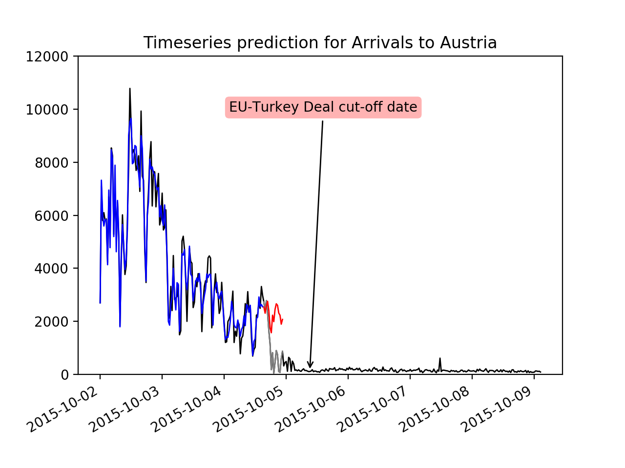
The UNHCR data consists of time series with daily arrival numbers of migrants in different countries. Its time window starts in October 1st 2015 and ends in April 23rd 2016. For the date March 20th 2016 an extra note is added, marking the events around the “EU-Turkey Deal”. Following this event, a clear structural break can be observed across several of the time series.
While we investigated on auto-correlation and several time series models such as various ARIMA models, LSTMs and Dynamic Linear Models, I stick to the multi-linear regression model as a simple introduction here. Linear regression is well studied, an established technique in statistics and used since dozens of years across various fields. As we are using multiple features derived from within a single and also across different time series, we are creating a linear regression with multiple explanatory variables but with one predicted variable. This must not be confused with a multivariate linear regression in which multiple variables are predicted. So what we will finally end up is a function $f$ with signature $f: \mathbb{R}^p\rightarrow\mathbb{R}$ in which $p\in\mathbb{N}$ is the number of features.
Aggregating observation windows to features for a multi-linear regression
We are given data (observations) from the UNHCR of a stochastic process $\{X_t\}_{t\in\mathbb{N}}$. Below you can find a python example in which we take a first glimpse at the observations from the csv (comma separated values) file. $\{X_t\}_{t\in\mathbb{N}}$ are a set of random variables with $X_t: \Omega\rightarrow\mathbb{R}$ and $\Omega$ being the sample space. The index $t$ denotes a discrete time index.
Given a time series we could predict the next value of the series simply given its previous value. A time series is then called a first-order stochastic process as the current observation $X_{t_c}$ of $\{X_t\}_{t\in\mathbb{N}}$ is only dependent on its previous observation $X_{t_c-1}$.
import pandas as pd
data_path = 'data/humdataorg-20160921-AnalysisofEstimatedArrivals-with-date.csv'
df = pd.read_csv(data_path)
df.head()
| Date | Arrivals to Italy | Arrivals to Greek Islands | Departures to mainland Greece | Arrivals to fYRoM | Arrivals to Serbia | Arrivals to Croatia | Arrivals to Hungary | Arrivals to Slovenia | Arrivals to Austria | |
|---|---|---|---|---|---|---|---|---|---|---|
| 0 | 10/1/2015 | 343 | 2631 | 2409 | 4370 | 5900.0 | 4344 | 3667.0 | 0.0 | 4550 |
| 1 | 10/2/2015 | 0 | 4055 | 1215 | 5853 | 3700.0 | 5546 | 4897.0 | 0.0 | 2700 |
| 2 | 10/3/2015 | 128 | 6097 | 4480 | 4202 | 3700.0 | 6086 | 6056.0 | NaN | 7100 |
| 3 | 10/4/2015 | 62 | 4763 | 1513 | 5181 | 4250.0 | 5065 | 5925.0 | 0.0 | 5800 |
| 4 | 10/5/2015 | 0 | 5909 | 7833 | 4282 | 3250.0 | 6338 | 5952.0 | 0.0 | 6100 |
This “first-order” assumption, however, is rather strict and most likely does not apply to the time series given by the UNHCR. We therefore considered multiple features of a time series window to predict a small forecasting horizon. The window with known observations is restricted to a finite number of $X_t$ preceeding the observation for forecasting. A feature aggregator is a function mapping this set of observations to an aggregated feature: $agg: \Omega\rightarrow\mathbb{R}, \omega \mapsto f_{agg}(\{X_w(\omega)\}{w\in\mathbb{N}})$ with $f{agg}: \mathbb{R}^w\rightarrow\mathbb{R}$ and $w\in\mathbb{N}, w\leq t$. Usually $w$ is a fixed window size.
An exemplary feature aggregator would be $agg_{avg}$ with $f_{agg_{avg}}(x) = \frac{1}{|x|}\sum\limits_{i=0}^{|x|} x_i$ which aggregates the observations over a window of $\{X_t\}_{t\in\mathbb{N}}$ into an averaged observation:
import numpy as np
series = 'Arrivals to Italy'
agg_avg = np.mean
agg_std = np.std

window_1 = (0, 200)
print(agg_avg(df[series][window_1[0]:window_1[1]]))
# = 231.01 (window1 mean)
print(agg_std(df[series][window_1[0]:window_1[1]]))
# = 445.2295 (window1 standard deviation)
print(df[series][window_1[1]])
# 343 (first value to predict after window 1)

window_2 = (50, 250)
print(agg_avg(df[series][window_2[0]:window_2[1]]))
# = 305.19 (window2 mean)
print(agg_std(df[series][window_2[0]:window_2[1]]))
# = 610.9442 (window2 standard deviation)
print(df[series][window_2[1]])
# 0 (first value to predict after window 2)
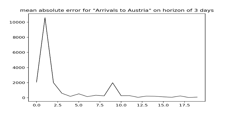
We defined multiple feature aggregators such as the mean, maximum, minimum, standard deviation, median or last seen value of a given window. For multiple time series of Italy, Serbia, North Macedonia (fYRoM), Greek Islands, mainland Greece, Croatia, Slovenia, Hungary and Austria we are given nine different observation series of stochastic processes of which we know that they somehow depend on each other. With six feature aggregators and nine windows of observations we obtain a feature set of $6\cdot 9 = 54$ features to predict a horizon (small window of the unseen data). By this method, we can train a multi-linear regression model for each time series (nine different models) and evaluate its performance with classical methods such as the mean absolute error and the R2 score. For each time series we obtain a final model $f_{country}: \mathbb{R}^{54}\rightarrow\mathbb{R}$ which is independent of any time index. To assess the quality of the model we train it on a sliding or increasing time window over the observations and measure the mean absolute error on a time horizon of e.g. three days. The assumption is, that the feature aggregations capture enough information to predict the next value.
Pros:
- easy to implement
- auto-correlation studies suggest almost stationarity
- error easy to understand
Cons:
- no knowledge outside one particular series itself
- no knowledge about outside events (see EU-Turkey deal)
- no considerations of spatial information at all
- no possibilities to change spatial resolutions
Simulation Experiments

Without getting too much into existing statistical models, we wanted to tackle some particular issues which we have not been familiar with before as technical partners in the Human+ project:
- the provided time series are clearly dependent on each other in some way and especially on some spatial dimension
- we want to incorporate prior knowledge such as spatial migration flow direction or give control over certain events into our models
- the provided spatial resolution on a country level is not sufficient for our project partners to actually work with in face of migration aid
So our thoughts went into the direction of trying to simulate migration. This triggered a discussion about the difference between a prediction / forecasting and a simulation. Despite open thoughts, we agreed on that a prediction model is providing a point estimate for the future (given prior knowledge and an observed path) while a simulation produces a possible sample path for the future or even over the past given some context knowledge about the underlying process.
As we will later see and as I indicated above with $\{X_t\}_{t\in\mathbb{N}}$, we are actually dealing with some kind of stochastic processes over finite time and finite states (countries). From a bayesian perspective this might already indicate the usage of a Hidden Markov model. But we will start with our initial considerations – not knowing of any markovian models – and slowly build the formalities up.
Important: Note, that we are now thinking about modeling actual counts and not the arrivals as provided by the UNHCR data. This will make our modeling very theoretical as we have only differential, erroneous and few observations available to verify our ideas.
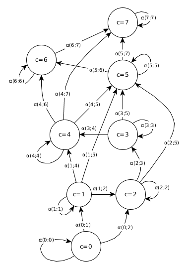
At each time step $t$ we observe for each time series a number of persons in a particular country. Having eight countries, we could represent this observation as $x_t = (100, 0, 0, 0, 0, 0, 0, 0)$, meaning that we observe 100 people in Greece and no people elsewhere. Assuming now, we would know of a deterministic process, deciding how persons from one country get distributed to another country. Then we would know an operation for the next time which maps $x_t$ to a new state vector $x_{t+1}$. For example, we could simply formulate this operation as a shift from one state to the “next” one and we would come up with $x_{t+1} = (0, 100, 0, 0, 0, 0, 0, 0)$.
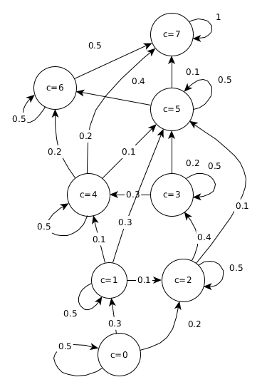
Furthermore, we do not want to reduce the total amount of observations when people transition from one state to the other. What we then come up with is a transition matrix which defines how people at one state are transitioning to another state. It can be formulated as $A\in\mathbb{R}^{c\times c}$ with $c\in\mathbb{N}$ being the number of states (and in our case countries). This transition matrix has the property of being column stochastic (see stochastic matrix), meaning that all entries of a column sum up to one. When we multiplicate our state vector $x_t$ with this transition matrix, we come up with the new state $x_{t+1}$. The matrix could look like the following: $$A = \begin{pmatrix}0.5 & 0 & 0 & 0 & 0 & 0 & 0 & 0\\0.3 & 0.5 & 0 & 0 & 0 & 0 & 0 & 0\\0.2 & 0.1 & 0.5 & 0 & 0 & 0 & 0 & 0\\0 & 0 & 0.4 & 0.5 & 0 & 0 & 0 & 0\\0 & 0.1 & 0 & 0.3 & 0.5 & 0 & 0 & 0\\0 & 0.3 & 0.1 & 0.2 & 0.1 & 0.5 & 0 & 0\\0 & 0 & 0 & 0 & 0.2 & 0.4 & 0.5 & 0\\0 & 0 & 0 & 0 & 0.2 & 0.1 & 0.5 & 1\end{pmatrix} $$ This transition matrix now states (informally) that 50% of people in Greece (state / country $c=0$) are staying in Greece, while 30% transition to $c=1$ and 20% transition to $c=2$. One could also view it more probabilistic and state, that with probability of 30% someone in Greece transitions to $c=1$. However, then the transition would be stochastic in contrast to the deterministically “known operation” as stated before, so we first consider it as deterministic. The difference is, that in the stochastic case we also could observe $x_{t+1} = (48, 28, 24, 0, 0, 0, 0, 0)$ instead of $x_{t+1} = (50, 30, 20, 0, 0, 0, 0, 0)$ and only “on average” we would observe it as the latter one in a probabilistic sense.
I) Computing or sampling the next state in the Graph
In this part we want to think about how to obtain a new possible state at time $t+1$ given the transition matrix and a state at time step $t$. As we came across several “issues”, I’m going to cover them in the same order in the following:
- Fast matrix-vector computation: we started off with a simple idea for computing the next state
- Issues & thoughts about real numbers instead of natural numbers
- Sampling from a multi-sided biased (or loaded) dice
Matrix-vector computation
Now, given a transition matrix $A$ and a state vector $x_t$ we can calculate the next observation as $x_{t+1} = A\cdot x_t$ (with $\cdot$ being the matrix multiplication). Before we continue extending our thoughts on how to build a simulation model about migration over discrete states and continuous output numbers, let’s first note some properties of this process. Each column vector of $A$ represents the distribution of a country to each other country. If each column vector is summing up to one, the matrix $A$ is column stochastic. Practically, this means that we do not “lose” any of the observed numbers when transitioning from one time step to the next. This means that the above matrix-vector-multiplication ensures that each $x_t$ has the same sum. Also, this gives some intuitions about transition matrices of Hidden Markov models over finite states. If the sum would be larger than one, the numbers would increase, if it would be smaller than one, the numbers would decrease in the next state vector. On the diagonal of the matrix we can observe self-loops of the graph. They are the transition values for each country to itself. You can imagine it as the probability of staying in the current country. As the exemplary matrix is a lower triangular matrix, it also represents a directed graph. If we would have entries in the upper triangular matrix, there would be also backwards directed edges. Now, iteratively applying $x_{t+1} = A\cdot x_t$ is actually a power iteration and as $A$ is a stochastic matrix the vector $x_t$ will converge against the eigenvector of $A$ (see Perron-Frobenius theorem). In case of our concrete $A$ it will even move all people from country $c=0$ to country $c=7$ as the graph of $A$ is directed forward and $c=7$ is the only sink with no outgoing edges except to itself.
If we now compute all state vectors for $A$ with an initial vector $x_0 = (100,0,0,0,0,0,0,0)$, we obtain the following:
x_c = np.array([100, 0, 0, 0, 0, 0, 0, 0])
for _ in range(30):
    x_c = np.dot(A, x_c)
    print(np.round(x_c, 2))
[50. 30. 20.  0.  0.  0.  0.  0.]
[25. 30. 23.  8.  3. 11.  0.  0.]
[12.5 22.5 19.5 13.2  6.9 18.7  5.   1.7]
[ 6.25 15.   14.5  14.4   9.66 21.38 11.36  7.45]
[ 3.12  9.38 10.   13.   10.65 20.49 16.16 17.2 ]
[ 1.56  5.62  6.56 10.5  10.16 17.72 18.41 29.46]
[ 0.78  3.28  4.16  7.88  8.79 14.32 18.32 42.47]
[ 0.39  1.88  2.56  5.6   7.09 11.01 16.65 54.82]
[ 0.2   1.05  1.55  3.82  5.41  8.15 14.15 65.66]
[ 0.1   0.59  0.92  2.53  3.96  5.85 11.42 74.64]
...
[ 0.    0.    0.    0.    0.    0.    0.   99.99]
[  0.   0.   0.   0.   0.   0.   0. 100.]
The result of our simulation is obviously a series of state vectors over time.
Natural numbers for simulation paths
We see, that all persons transitioned from $c=0$ to $c=7$ after 30 discrete time steps. However, we now notice, that we have floating points in our state vectors but we actually want a simulated path of observed people, so our state output should be continuous but within the natural numbers.
We tackled several variants to solve this issue. The first idea was to distribute people in each state by the transition probability and rounding the numbers. Variant A1 and A2 describe two possibilities to use the transition probabilities in this “hard” computational style. Variant B explains a better (probabilistic) approach in which each person in a state is actually choosing the next state based on the transition probabilities.
Variant A1: distributing people in to new states with “hard” transitions
Partitioning $n\in\mathbb{N}$ into $k_1,\cdots,k_p\in\mathbb{N}$ with $a_1,\cdots,a_p\in(0,1)$ and $\sum_{i=1}^p a_i = 1$ such that $\sum\limits_{i=1}^p a_i\cdot k_i = n$ is not solvable for arbitrary $a_i$. To still enforce entries in $x_t$ to be natural numbers, we applied a trick which introduces some randomness. For a particular country and their observed people, we compute the rounded number of people for all transitions from that country until the sum exceeds the original value. Then we fill up the last transition with the difference of the observed people and the sum of the rounded numbers. As this introduces an error to the last transition, we choose a random order in which we consider the transitions.
For state $c$ a random permutation of $A_{c}$ is computed and its partition of $x_{t,c}$ is successively subtracted.
E.g. for $c=0$ we obtain $A_0 = (0.5, 0.3, 0.2, 0, 0, 0, 0, 0)$ and after discarding zero-valued entries we obtain a random permutation $\pi_{t,c} = (0.3, 0.2, 0.5)$.
The value $x_{t=0,c} = 100$ is then successively divided into $k_0 = \lfloor0.3\cdot 100\rceil = 30, k_1 = \lfloor0.2\cdot 100\rceil = 20, k_2 = 100-(k_0+k_1) = 50$.
For natural numbers, not equally partionable by $A_0$, such as $25$ we would obtain $k_0 = \lfloor0.3\cdot 25\rceil = 8, k_1 = \lfloor0.2\cdot 25\rceil = 5, k_3 = 25-(8+5) = 12$.
Now, our previous time-step operation $x_{t+1} = A\cdot x_t$ gets pretty complicated as we can not rely on this matrix operation any more and have to compute a random permutation.
The below code partitions a number n into buckets of natural numbers according to a partitioning defined in a.
def get_partition(n, a):
    assert np.equal(np.sum(a), 1)
    partitions = np.zeros(len(a))
    if n < 1:
        return partitions

    permutation = np.random.permutation(len(a))
    p_idx = 0
    current_sum = 0
    while current_sum < n and p_idx < len(a)-1:
        a_k = a[permutation[p_idx]]
        new_summand = np.round(a_k*n)
        if new_summand < n-current_sum:
            partitions[permutation[p_idx]] = new_summand
            current_sum += new_summand
        else:
            break
        p_idx += 1

    if current_sum < n:
        while p_idx < len(a)-1 and a[permutation[p_idx]] == 0:
            p_idx += 1
        partitions[permutation[p_idx]] = n-np.sum(partitions)

    assert np.equal(np.sum(partitions), n)
    return partitions
Now we can compute each step with our new distribution operation for a particular country:
x_c = np.array([100, 0, 0, 0, 0, 0, 0, 0])
for _ in range(30):
    x_c = np.sum(
      [get_partition(v, A[:,ix]) for ix, v in enumerate(x_c)
    ], axis=0)
    print(x_c)
print(x_c)
The output looks (closely) like:
[50. 30. 20.  0.  0.  0.  0.  0.]
[25. 30. 23.  8.  3. 11.  0.  0.]
[12. 23. 20. 13.  7. 19.  4.  2.]
[ 6. 16. 14. 14. 10. 23. 10.  7.]
[ 3. 10. 10. 13. 10. 22. 16. 16.]
[ 1.  6.  7. 10. 10. 19. 19. 28.]
[ 0.  3.  5.  7.  9. 16. 20. 40.]
[ 0.  2.  2.  6.  6. 11. 18. 55.]
...
[ 0.  0.  0.  0.  1.  0.  0. 99.]
[ 0.  0.  0.  0.  0.  0.  1. 99.]
[  0.   0.   0.   0.   0.   0.   0. 100.]
[  0.   0.   0.   0.   0.   0.   0. 100.]
We now enforced, that each $x_t$ can only contain natural numbers and that the sum of all observations has to stay equal as long as the matrix $A$ is column stochastic.
Variant A2: using matrix-vector computation with little random errors
A way easier approach with similar results is by still using the matrix-vector multiplication $A\cdot x_t$, but directly using rounding on that result.
Rounding makes sure we get from real to natural numbers, however, it is now possible that we introduce errors.
So we simply compute the difference to the original sum of people in all states, see x_sum0.
Then, a random state from the graph is selected and the difference is subtracted from that random state.
We choose a non-zero state from the vector x_c to increase the probability catching a state which was involved in the transition, because only states in which people are left after the transition computation could have been involved in the transition.
x_c = np.array([100, 0, 0, 0, 0, 0, 0, 0])
x_sum0 = np.sum(x_c)
for _ in range(30):
    x_c = np.round(np.dot(A, x_c))
    diff = np.sum(x_c)-x_sum0
    random_nonzero_idx = np.random.choice(np.nonzero(x_c)[0])
    x_c[random_nonzero_idx] -= diff
    print(x_c)
[50. 30. 20.  0.  0.  0.  0.  0.]
[25. 30. 23.  8.  3. 11.  0.  0.]
[12. 22. 20. 13.  7. 19.  5.  2.]
[ 6. 14. 15. 14. 10. 21. 12.  8.]
[ 3.  9. 10. 13. 11. 20. 16. 18.]
[ 2.  5.  6. 12. 10. 17. 18. 30.]
[ 1.  3.  4.  8.  9. 14. 18. 43.]
[ 0.  2.  2.  6.  7. 11. 16. 56.]
[ 0.  1.  1.  4.  6.  8. 14. 66.]
[ 0.  0.  1.  2.  4.  7. 11. 75.]
[ 0.  0.  0.  1.  3.  4.  9. 83.]
[ 0.  0.  0.  0.  2.  3.  7. 88.]
[ 0.  0.  0.  0.  1.  2.  5. 92.]
[ 0.  0.  0.  0.  0.  1.  4. 95.]
[ 0.  0.  0.  0.  0.  0.  2. 98.]
[ 0.  0.  0.  0.  0.  0.  1. 99.]
[  0.   0.   0.   0.   0.   0.   0. 100.]
We did not invest more time into investigating on the differences between both methods. The second one clearly has its computational benefits, however it also adds noise to randomly selected countries. On the other hand, the first method distributes deterministically among the outgoing edges and only randomizes on which the rounding happens.
Variant B: throwing a die
The transition probabilities of one state, e.g. $a_0 = [0.5, 0.3, 0.2, 0, 0, 0, 0, 0]$, actually suggest to draw from a distribution.
But what distribution do we draw from?
What is the random variable?
For a single person at state $c = 0$, the transition probabilities $a_0$ specify that the person stays in the current state with a probability of 50%.
With 30% probability the person transitions to $c = 1$ and with 20% probability to $c = 2$.
This is equivalent to throwing a loaded die.
With numpy, a single result of such a die throw can be obtained with np.random.choice.
If now $n=100$ pepople are transitioning, we have to collect the target states after one hundred such loaded die throws:
def roll(n:int, a):
    choices = [k for k,v in enumerate(a)]
    buckets = {k: 0 for k in choices}
    for i in range(n):
        buckets[np.random.choice(choices, p=a)] += 1
    return [buckets[k] for k in choices]
A possible output looks like:
roll(100, [0.5, 0.3, 0.2, 0, 0, 0, 0, 0])
[55, 25, 20, 0, 0, 0, 0, 0]
Using this approach, we get the following simulated state vectors:
x_c = np.array([100, 0, 0, 0, 0, 0, 0, 0])
for _ in range(30):
    x_new = np.zeros(x_c.shape)
    for country_pop, outgoing_probs in zip(x_c, A.T):
        x_new += roll(int(country_pop), outgoing_probs)
    x_c = x_new
    print(x_c)
We obtain:
[38. 39. 23.  0.  0.  0.  0.  0.]
[17. 34. 22.  8.  5. 14.  0.  0.]
[ 7. 23. 20. 12.  8. 19.  7.  4.]
[ 4. 14. 10. 18.  5. 25. 18.  6.]
[ 2.  5.  4. 17.  9. 27. 19. 17.]
[ 2.  3.  2. 10.  9. 20. 25. 29.]
[ 0.  2.  2.  6. 10. 15. 21. 44.]
[ 0.  1.  1.  5.  7. 13. 19. 54.]
[ 0.  1.  0.  4.  7.  6. 20. 62.]
[ 0.  1.  0.  3.  4.  3. 14. 75.]
[ 0.  0.  0.  2.  4.  3.  7. 84.]
[ 0.  0.  0.  1.  3.  3.  4. 89.]
[ 0.  0.  0.  1.  1.  2.  2. 94.]
[ 0.  0.  0.  0.  1.  2.  2. 95.]
[ 0.  0.  0.  0.  1.  2.  1. 96.]
[ 0.  0.  0.  0.  1.  1.  2. 96.]
[ 0.  0.  0.  0.  0.  0.  3. 97.]
[ 0.  0.  0.  0.  0.  0.  1. 99.]
[  0.   0.   0.   0.   0.   0.   0. 100.]
What we came up here with is actually a multinomial distribution, the generalization of the binomial distribution in which a $k$-sided dice is rolled $n$ times.
Given the example above with $n = 100$ and our $k = 8$ sided dice with $a_0 = [0.5,0.3,0.2,0,0,0,0,0]$ as our probabilities for the multinomial distribution, we can also easily call np.random.multinomial to roll our dice:
np.random.multinomial(100, [0.5, 0.3, 0.2, 0, 0, 0, 0, 0])
array([55, 29, 16,  0,  0,  0,  0,  0])
II) Defining (prior) transition probabilities in $A$
Now that we have a transition operation for consecutive discrete time steps with strict natural numbers for our output, we continued with ideas on how to define transition probabilities in the matrix $A$. At this point, I assume that we are pretty much abusing probabilistic ideas in context of Hidden Markov models. For a Hidden Markov model with a transition and an emission matrix those information could be learned with the Baum-Welch and the Viterbi Algorithm, but we a) had no direct observations to learn from and b) we wanted to introduce real-world knowledge into the “model”. Therefore, we followed a first idea of initializing the transition probabilities with inverse distances of the actual countries and restricted edges of the graph to those which are within a limited distance. In a later step, we think about how to adapt the transition probabilities when seeing new data.
Geographic distances to initialize transition probabilities
We are interested in using real-world information for modeling migration flow. For this, we thought about online available information such as
- the geographic distance between nodes (cities, countries, regions)
- the types of infrastructure available between nodes such as trains, bus or flight connections, highways and roads
- trajectories from social media (independently a part of our research project Human+)
At first, we investigated on using the geographic distance $d_g(u, v)$ between two nodes $u$ and $v$. One idea was to simply use the inverted distance between two nodes as the transition probability. This reflects the assumption that people transition with lower probability between nodes far apart from each other. For a set of nodes $V$ (commonly standing for “vertices” in graph theory) we simply defined the transition matrix as $A_{ij} = \frac{1}{d_g(i,j)}$ for $i,j\in V$ and then normalized the sum of probabilities leaving from one node to equal one (to ensure, we keep our column stochasticity). Depending on where we take the data from, we might likely come up with a high density of connections between nodes in the graph. We took data from Open Street Map (OSM) for auto-generated graphs but mostly tested our simulation experiments with small manually defined graphs. In the case of large auto-generated graphs from OSM data, we defined lower and upper limits for distances. This reflects our assumption that people cover only up to a limited geographic distance per time step (e.g. one day). Defining a probability for the recurrence connection for each state seemed very arbitrary to me and we initially mostly set it to a custom value such as 0.5.
Multiple factors for transition probabilities
As we’ve seen above, there are various ways and assumptions to model a prior probability of how likely it is to transition from one node to another node. If we have inverse distances, we easily can come up with weights for each outgoing edge of a single node in the graph. But if we have $f\in\mathbb{N}$ factors $q_1,\dots,q_f$ for a particular outgoing edge, how do we combine them into a transition prior probabilty? We first assume each factor to represent a probabilty, thus $\forall i\in\{1,\dots,f\}: q_i\in(0,1)$. In case of distances between geographic nodes, we simply had one “geographic distance” factor $q_{geo\_dist} = \frac{1}{d_g(u,v)}$. To be slightly more precise, a factor is actually a function $q: V\times V\rightarrow(0,1)$, providing a probability for transitioning from $u$ to $v$. Furthermore, we let each factor with source node $u$ sum up to one. For the geographic distance, we scaled the inverted distances to sum up to one. By this definition, we can easily combine factors e.g. in a uniform manner by adding them.
Imagine four real-world factors $f_1, f_2, f_3, f_4$ for a node with 3 outgoing edges:
f1 = np.array([0.2, 0.7, 0.1])  # f_1(u,[v1,v2,v3])
f2 = np.array([0.3, 0.1, 0.6])  # f_2(u,[v1,v2,v3])
f3 = np.array([0.1, 0.1, 0.8])
f4 = np.array([0.2, 0.5, 0.3])
We can easily combine them uniformly:
(f1+f2+f3+f4)/4
array([0.2 , 0.35, 0.45])
If we imagine different weights $fw_1=0.1, fw_2=0.2, fw_3=0.6, fw_4=0.1$ for each factor, we could also get:
(0.1*f1+0.2*f2+0.6*f3+0.1*f4)
array([0.16, 0.2 , 0.64])
But how much influence does which factor have? Assuming, each factor could influence not just the prior probability but also the learning step when changing this transition probabilities, we could think of the factors coming from another probability. The underlying distribution for this could be the Dirichlet distribution. Often, this distribution is also called a distribution over distributions (although we’re more talking about discrete distribtions than general distributions). What is the Dirichlet distribution?
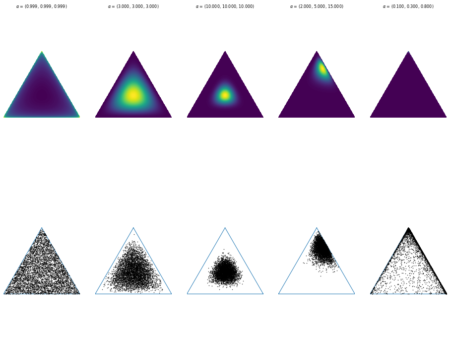
The Dirichlet distribution is parameterized by $\alpha$, a vector of real values. For $\alpha = (\alpha_1, \dots, \alpha_k)$ the distribution provides samples of real values $x_1,\dots,x_k$ with $x_i \in (0,1)$ and all of those $x_i$ summing up to one.
Now, we can use this distribution to represent our belief about the weight distribution of our real-world factors influencing the transition probability of our graph. Low values can be used to represent uncertain beliefs for some factors, while the proportions of $\alpha$ values reflect the proportion of influence of each factor. If the belief of our model is pretty uncertain, the sampled factor weights will have a high variance and we will have a high stochasticity for our transition probabilities. Learning should contribute in stabilizing those factor weights by getting more and more sure about the Dirichlet parameters.
III) Parameters of the simulation model
Given a fixed transition graph $A$ given, power iteration of an initial state vector $x$ converges to some eigenvector as explained above. In other words, people will pretty much traverse the graph in the same manner based on a constant transition matrix and an initial state vector $x_0$. Only with changes in each step provides changes in the simulation series over time. If those changes are deterministic, the whole process again, behaves deterministic. This is why we need to introduce some stochasticity into the model. However, we want to avoid ignorant randomness as we still would like to sample realistic paths of walks through the graph. What options do we have to parameterize our model? We came up with following options to adapt the simulation model:
- Given a country $c$, new people could randomly arrive or depart, e.g. by a poisson distribution. This could also be restricted to only selected “entering” or “exiting” countries. So, for each country we could learn the parameters of a poisson distribution (or any other process yielding entering/exiting numbers for countries).
- In each time step the transition probabilities could be changed, e.g. by small errors (noise) or by events related to the particular time step. Given observations, parameters for adding small noise (e.g. from a normal distribution) could reflect uncertainty of the process within a single time step. One could learn “global” parameters for a single normal distribution disturbing each step or “local” parameters for normal distributions per time step.
- The transition probabilities per country could also be made stochastic themselves, viewing them as a sample from a Dirichlet distribution and only the parameters of this distribution could be learned / stabilized across multiple time steps. This matches with the section on multiple factors for transition probabilities.
IV) Evaluating the model
Once more, it is important to mention at this point, that the data available from the UNHCR are daily arrivals for selected countries on the Balkan route between 2015 and 2016. Thus, only differences for consecutive time steps are available. I assume, this calls loudly for modeling the data with (stochastic) differential equation (SDE). However, I am neither familiar with modeling and fitting SDEs nor do I know of any possibility to connect them over multiple time series – which obviously have dependencies among eachother. So, assuming I have a sampled series of observations per state (country), the main idea I came up so far was to run the simulation, calculate differences for each time step and use a selected measure to relate it to the available UNHCR data.
What does running the simulation now mean? It basically means sampling a single concrete path for a finite number of steps by following the above sketched steps. We decide on a concrete version of the simulation model. At first, geographic regions are selected as units for the underlying graph. We can have regions with different spatial resolution. The transition matrix $A$ is initialized from real-world factors such as geographic distances. The initial state (number of people at a particular country) is initialized from the UNHCR data e.g. by assuming that the arrivals at the first given observation equal the total sum. Then, for each time step the power iteration is computed. Optionally, disturbance or event values are added per time step. Arrival or departure values are calculated per time step.
In a time series cross validated manner, the simulation then runs over $h_{sim}=30$ time steps. Over this training window a measurement would be calculated. This could be e.g. a correlation coefficient between the simulated path differences and the actual observations from the UNHCR data fitting this time window. Then we move the window forward and repeat the computation. The aggregated (e.g. averaged) correlation gives a statistic of how well the simulation model aligned with the actual observation based on the initial parameter set. Some of the parameters, e.g. number of initial people at several countries, would be inferred from daily arrival numbers from the UNHCR data. After a whole run over e.g. a window of $h_{train} = 200$ steps (= days) and shifting the simulation window e.g. one step after each other, we obtain an aggregated statistic on how well the simulation model with our initial parameter set worked out. Then, we adapt parameters with respect to an optimization strategy. The initialization parameters such as the initial state for comparing it with the UNHCR data will be kept constant. As naive optimization strategy, a random search over the concerned parameters could be selected. I could not come up with an idea of how to link e.g. a gradient descent method to it and probably with so few data points, it probably does not even matter. On the other hand, I found that CMA-ES works pretty fine for low-dimensional optimization. Furthermore, given that we know about properties of the distributions used in the model, we could also employ ideas from genetic algorithms to optimize (learn) model parameters until we sample realistic migration flows given some evaluation metric. As long as our concrete simulation model has only few dimensional parameters, we can employ such population based optimization techniques over random sampling with the cost of memory requirements.
Sketch of this learning procedure:
data = UNHCR
population = set(SimulationModel(params) for random(params))
num_generations = 100
evaluations = map()
for current_generation : num_generations:
	evaluate(population, data)
	mutation(population)
	selection(population)
	crossover(population)
	sample_random(population)