Part of the Big Picture of my PhD is analyzing and interpreting the graph theoretic properties of computational graphs of Artificial Neural Networks. But what is that computational graph and how is it defined? And what’s an Artificial Neural Network in that context? When thinking of numerical frameworks for computational graphs such as PyTorch or Tensorflow, do we talk about the same computational graph? This post is about trying to formulate some of my thoughts about that questions.

Without going into areas such as optimization (“how to find/train parameters of a model?"), without thinking about topological properties of data or without prior assumptions on data (“how is unseen data distributed?"), I simply start defining Artificial Neural Networks (ANNs) as a function space with certain restrictions over contained functions. Over this function space we later can define computational graphs on different levels (or orders).

For this, we

1. formulate the usual notion of a neuron, layers and an Artificial Neural Network as a whole
2. show how some notations make restrictions to the Artificial Neural Network
3. have a look at the whole computational graph of a model

Artificial Neural Networks

The formalization of ANNs stems from biological inspiration of neurons. Biological neurons accumulate incoming signals and propagate a signal as soon as a threshold is exceeded. Mathematical formulations for Artificial Neural Networks do not consider any continuous time or any signal processing in that sense. Models that respect such properties are e.g. Spiking Neural Networks. From a mathematical perspective, an ANN is nothing more than a function composed of non-linear elements – neurons and their connections – which can learn from data and then solve a regression or classification task.

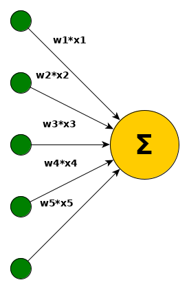
The idea of a neuron can now mathematically be represented with $f_w(x) = \sum\limits_{i=0}^{d_1} w_i\cdot x_i$ with $w, x\in\mathbb{R}^{d_1}, d_1\in\mathbb{N}, f: \mathbb{R}^{d_1}\rightarrow\mathbb{R}$. For now, simply assume that we somehow come up with an adequate $w$ to solve a particular classification or regression problem (finding the weights $w$ is the process of learning).

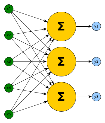
Each incoming signal (or better value in that sense) is weighted and the whole weighted incoming information is summed up. So far, the neuron is a linear transformation of $x$. To solve non-linear problems, the model must be able to represent non-linearities. Otherwise it simply performs only linear operations such as scaling or rotations. Thus, a thresholding mechanism and a shifting value (bias) is introduced. This part is called an activation. While each incoming value could be thresholded with different sigmoid functions, it is common to use the same one for all neurons. The formalisation then changes from $f_w(x) = \sum\limits_{i=0}^{d_1} \sigma_i(w_i\cdot x_i+b_i)$ to $f_w(x) = \sigma(\sum\limits_{i=0}^{d_1} (w_i\cdot x_i)+b)$. Multiple neurons in the model are simply multiple $f_w$ with different $w$ reacting to the same input $x$. So far, the formalisation of ANNs is pretty straight-forward and can be found across different literature.

At this point, multiple neurons are usually bundled together. Having input $x\in\mathbb{R}^{d_1}$ and $d_2\in\mathbb{N}$ neurons with above non-linear weight-summing functions, one obtains weights $w_{j,i}\in\mathbb{R}^{d_2\times d_1}$. The function of an Artificial Neural Network then maps from an input space $x\in\mathbb{R}^{d_1}$ to an output space $\mathbb{R}^{d_2}$. Usually $d_1$ is way larger than $d_2$. In case of image classification problems such as MNIST $d_1$ equals the possible pixel amount, e.g. $d_1 = 28\times28 = 784$, while $d_2$ is the number of possible classes in that task, e.g. the number of possible digits $d_2 = 10$. Given, that all neurons use the same activation function but with different biases, the function definition changes to $f_W(x) = \sigma(W\cdot x+b)$ with $W$ being the $d_2\times d_1$-matrix containing the weights $w_{i,j}$ and $\cdot$ being the dot-product-operator. That way, the formulation looks already pretty clean. Multiple neurons with the same input can be bundled together in a linear algebra way with a matrix-vector notation. By the way: this also shows the GPU-friendlyness as those computer architectures are specially designed for efficient and parallel matrix-vector multiplications. The notation, however, requires already some structural properties such as having the same activation function for all neurons. And as soon as we are stacking multiple layers, these requirements grow further.

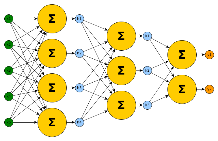
Now, to get closer to the design of todays architectures of Artificial Neural Networks, multiple such non-linear learnable functions $f_w$ get stacked.

Given a finite series $(a_i)_{i\in{0,\dots,l}}$ with $a_i\in\mathbb{N}$ and $a_0=d_1$ and $a_l=d_2$ we can define an Artificial Neural Network $ANN: \mathbb{R}^{a_0}\rightarrow\mathbb{R}^{a_l}$ as a composition of $(f_i)_{i\in{1,\dots,l}}$. Those $f_i: \mathbb{R}^{a_{i-1}}\rightarrow\mathbb{R}^{a_{i}}$ are defined as above and each has parameters $W_i$ and $b_i$. The composition is then for each layer $i$ a function $g_i$: $\forall i\geq 2: g_{i}(x) = f_{i}(g_{i-1}(x))$ with $g_1$ being $f_1$ and the signature of $g_i: \mathbb{R}^{a_{i-1}}\rightarrow\mathbb{R}^{a_i}$ matches the one of $f_i$. We then set $ANN(x) = g_l(x)$.

As an example, we could have the finite series $a_0 = 784, a_1 = 200, a_2 = 100, a_3 = 10$ with $l = 3$. Then the layer-wise grouped neuron functions $f_1(x) = \sigma(W_1\cdot x+b_1)$, $f_2(x) = \sigma(W_2\cdot x+b_2)$, $f_3(x) = \sigma(W_3\cdot x+b_3)$ get composed to $g_1(x) = \sigma(W_1\cdot x+b_1)$, $g_2(x) = \sigma(W_2\cdot \sigma(W_1\cdot x+b_1)+b_2)$ and $g_3(x) = \sigma(W_3\cdot \sigma(W_2\cdot \sigma(W_2\cdot x+b_2)+b_2)+b_3)$. The final ANN has then the signature $ANN: \mathbb{R}^{784}\rightarrow\mathbb{R}^{10}$ with $ANN(x) = g_3(x)$.

So far, most classical Artificial Neural Networks can be represented with this compositional structure. But todays ANNs consist of way more techniques than only linear transformations and activation functions. From an architectural perspective there exist ideas such as Convolutions, Dropout, Pooling, Capsules or Skip-Layer Connections and beyond architectural considerations there are data augmentation, loss function definitions, regularization and many more things to ponder about.

TODO

• skip-layer connections and why ResNets use blocks as a trick
• viewing ConvNets as sparse connected layers with weight sharing
• dropout are fully connected layers with stochasticity
• pooling are structured layers with fixed weights
• capsules are structured layers with learnable weights
• idea: compiling networks into graphs back and forth for network analysis