Problem: obtain real-world statistics and process them into a graph
Solution: geopandas, shapely, rasterio, nominatim, osm-router
Incorporating real-world information into models is non-trivial. It is often done in machine learning by e.g. training models on natural images. In this post, I collect some notes and information on processing geographic statistics. Those statistics are then used in a geographically based model as described in a previous post about thoughts on simulating migration flow. Namely, I used geographic distances and population densities to initialize prior beliefs for a simulation model. Distances are computed with OpenStreetMap osm-router and population densities are obtained through NASA Earth Observations (for which you have to register, see ref-1). Furthermore, the Nomenclature of Territorial Units for Statistics (NUTS) is used to work with region hierarchies and to resolve geometries (see ref-2).
Ways for pre-defining geographical nodes
Goal: we want to build a statistical model based on a graph in which nodes represent geographical regions. How do we come up with the set of nodes or even the graph structure?
There are three proposed ways to proceed:
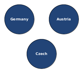
- Manually defining nodes of the graph. We use this approach as a demonstration of a valid graph.
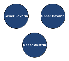
- Using the NUTS hierarchy to come up with a large set of nodes at a certain spatial resolution within Europe.
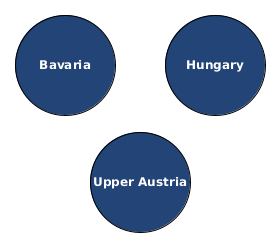
- Using geographical coordinates for reverse geo-coding and obtain nodes dynamically from user-defined selections.
For prototyping and experimental purposes, I usually manually defined a small set of nodes which represented a certain geographic region. In context of building a graph for migration flow simulation I used the countries of the Balkan route mentioned in the UNHCR dataset: Italy, Serbia, North Macedonia (fYRoM), Greek Islands, mainland Greece, Croatia, Slovenia, Hungary and Austria. For calculating concrete simulation paths for the Human+ project, I also used selected NUTS Level 2 regions as nodes, e.g. Lower Bavaria. They were also mixed with nodes of lower spatial resolution, such as the mentioned countries.
nodes = [ 'Italy', 'Serbia', 'North Macedonia', 'Greece', 'Croatia', 'Slovenia', 'Hungary', 'Austria' ]
Later, we will use this set of nodes and connect them to a graph.
Downloading the NUTS shapes from Eurostat and using geopandas gives us quickly information on regional hierarchies in Europe. Note, that I used SRID=4326 as the spatial reference system.
import os
import geopandas as gpd

nuts_base_path = 'data/nuts-codes'
shapefile_nuts0 = os.path.join(nuts_base_path, 'NUTS_RG_01M_2016_4326_LEVL_0.shp/NUTS_RG_01M_2016_4326_LEVL_0.shp')
shapefile_nuts1 = os.path.join(nuts_base_path, 'NUTS_RG_01M_2016_4326_LEVL_1.shp/NUTS_RG_01M_2016_4326_LEVL_1.shp')
shapefile_nuts2 = os.path.join(nuts_base_path, 'NUTS_RG_01M_2016_4326_LEVL_2.shp/NUTS_RG_01M_2016_4326_LEVL_2.shp')
shapefile_nuts3 = os.path.join(nuts_base_path, 'NUTS_RG_01M_2016_4326_LEVL_3.shp/NUTS_RG_01M_2016_4326_LEVL_3.shp')

# Resolve countries into shapes
nuts0_shapes = gpd.read_file(shapefile_nuts0)
nuts1_shapes = gpd.read_file(shapefile_nuts1)
nuts2_shapes = gpd.read_file(shapefile_nuts2)
nuts3_shapes = gpd.read_file(shapefile_nuts3)
Geopandas can be easily used to select geometries from the provided NUTS database.
The loaded geopandas dataframe objects contain several columns for each NUTS code: nuts0_shapes.columns gives me Index(['LEVL_CODE', 'NUTS_ID', 'CNTR_CODE', 'NUTS_NAME', 'FID', 'geometry'], dtype='object').
You can inspect it quite nicely within a jupyter notebook:
dataframe_germany = nuts0_shapes[nuts0_shapes['NUTS_ID'] == 'DE']
dataframe_germany.geometry.values[0]

Now, we can easily select all level-2 codes given some country codes:
nuts2_shapes[nuts2_shapes['CNTR_CODE'].isin(['DE', 'AT'])].head()
| LEVL_CODE | NUTS_ID | CNTR_CODE | NUTS_NAME | FID | geometry | |
|---|---|---|---|---|---|---|
| 5 | 2 | DE13 | DE | Freiburg | DE13 | MULTIPOLYGON (((8.22201 48.60323, 8.21404 48.6... |
| 7 | 2 | AT32 | AT | Salzburg | AT32 | POLYGON ((13.30382 48.00782, 13.30366 48.00400... |
| 12 | 2 | AT11 | AT | Burgenland | AT11 | POLYGON ((17.16080 48.00666, 17.13656 47.99510... |
| 14 | 2 | AT33 | AT | Tirol | AT33 | MULTIPOLYGON (((10.45444 47.55580, 10.47320 47... |
| 15 | 2 | DE14 | DE | Tübingen | DE14 | POLYGON ((10.23078 48.51051, 10.23266 48.50851... |
nodes = list(nuts2_shapes[nuts2_shapes['CNTR_CODE'].isin(['DE', 'AT', 'HU', 'RS', 'HR', 'HE', 'IT', 'MK', 'SL'])]['NUTS_ID'])
Output:
['DE13', 'AT32', 'AT11', 'AT33', 'DE14', 'AT34', 'DE21', 'AT22', 'AT12', 'AT13', 'AT21', 'DE11', 'DE22', 'DE12', 'AT31', 'DE73', 'DE40', 'DE93', 'ITH3', 'DEB1', 'DE94', 'DEB2', 'DE80', 'DEA3', 'DE24', 'DE27', 'DE71', 'DE91', 'ITG1', 'DEA4', 'DE25', 'ITG2', 'ITH1', 'DE72', 'ITH2', 'DE92', 'DEA5', 'DE23', 'DE26', 'DEA1', 'DEB3', 'DED2', 'DE30', 'DE50', 'DE60', 'DED4', 'DEA2', 'DEC0', 'DEE0', 'DEG0', 'DED5', 'DEF0', 'HR03', 'HR04', 'HU11', 'MK00', 'ITI1', 'ITI2', 'ITI3', 'ITI4', 'ITH4', 'ITH5', 'RS12', 'RS22', 'RS11', 'RS21', 'HU31', 'ITF1', 'ITF2', 'ITC1', 'ITC2', 'ITC4', 'ITF3', 'HU23', 'HU12', 'HU32', 'HU33', 'ITF4', 'HU21', 'ITF5', 'ITF6', 'HU22', 'ITC3']
There would now also be the possibility to reverse geocode a list of given coordinates, e.g.
points_of_interest = [
	(48.567, 13.449), # Passau
	(48.200, 16.400), # Vienna
	(46.047, 14.501) # Ljubljana
]
The difficult part of this is not the reverse geocoding (which is solved by existing systems such as OSM Routing), but resolving a set of points into non-intersecting regions. This problem probably matches the largest empty sphere or variants of it from computational geometry and could be covered in an own post. The goal would be to resolve a mixed set of regions, which cover the largest possible area without intersecting each other and maybe also respecting overall size restrictions. Given the NUTS hierarchy, it could also be mapped back into political regions.
Calculating distances for nodes
I used geographic distances for two purposes. The first purpose is to obtain an initial structure of the simulation graph. Basically, I am simply taking the nodes from the previous step such as “Italy”, “Serbia”, and so on and connect them as a graph with edges based on whether they have a route between each other and this route is within a certain distance. The structure of the graph is actually already a prior assumption on the model and at this step we simply want to have an objective tool which defines whether two nodes are connected (having a “1” in the adjacency matrix) or not (being “0” in the adjacency matrix of the graph). The second purpose would be to use the distance between geographic nodes as one of multiple possible real-world factors to define the weight of an edge between the respective nodes of the graph. In this purpose, the geographic distance would not only reflect as “1” or “0” in the adjacency matrix but actually has a more fine-grained influence on the weight, which represents a transition probability.
Goal: obtain a connection structure for our graph or even get distance information between nodes to use them as factors for weights.
For these purposes, I installed a local version of the Open Source Routing Machine which is a pretty nice project working with data of Open Street Map.
Goal: calling a local routing service to avoid using online (quota-limited) services:
curl 'http://localhost:5000/route/v1/driving/7.436828612,43.739228054975506;7.417058944702148,43.73284046244549'
Installing OSRM
These steps follow the official documentation at github.com/Project-OSRM/osrm-backend.
OSRM service needs open street map data. You can obtain e.g. data for Europe or Germany from download.geofabrik.de:
$ wget http://download.geofabrik.de/germany-latest.osm.pbf -O /media/data/osrm/germany-latest.osm.pbf
$ ls -l /media/data/osrm/
-rw-r--r-- 1 julian julian 22668184759 Mär 16 00:55 germany-latest.osm.pbf
Extract the pbf-file with a service provided by the osrm-backend image available on docker.
OSRM docker image is available at https://hub.docker.com/r/osrm/osrm-backend/tags and you can choose the latest version.
For me that was v5.22.0.
I mapped the host directory /media/data/osrm/ to the docker container’s directory /data and thus provided the file /media/data/osrm/germany-latest.osm.pbf which was previously downloaded.
Below steps can now be executed from outside of the container or within the container.
You can go into the container by executing docker run -i -t -v /media/data/osrm/:/data osrm/osrm-backend:v5.22.0
Notice, that the extraction might take a lot of RAM. I was not able to easily extract the files for europe, so I decided to go with an example for germany. The docker container crashed several times quietly and for germany the osrm-extract process stated at the end that it used around 9.4GB of RAM.
Calling the extraction on a given .osm.pbf-file:
$ docker run -t -v /media/data/osrm/:/data osrm/osrm-backend:v5.22.0 osrm-extract -p /opt/car.lua /data/germany-latest.osm.pbf
[info] Parsed 0 location-dependent features with 0 GeoJSON polygons
[info] Using script /opt/car.lua
[info] Input file: germany-latest.osm.pbf
..
[info] Processed 32689774 edges
[info] Expansion: 127853 nodes/sec and 78946 edges/sec
[info] To prepare the data for routing, run: ./osrm-contract "/data/germany-latest.osrm"
[info] RAM: peak bytes used: 10057203712
I obtained:
$ ls -l /media/data/osrm/
/media/data/osrm/germany-latest.osrm
/media/data/osrm/germany-latest.osrm.cnbg
/media/data/osrm/germany-latest.osrm.cnbg_to_ebg
/media/data/osrm/germany-latest.osrm.ebg
/media/data/osrm/germany-latest.osrm.ebg_nodes
/media/data/osrm/germany-latest.osrm.edges
[..]
/media/data/osrm/germany-latest.osrm.turn_weight_penalties
Creating the hierarchy, running osrm-contract:
$ docker run -t -v /media/data/osrm/:/data osrm/osrm-backend:v5.22.0 osrm-contract /data/germany-latest.osrm
[info] Input file: /data/germany-latest.osrm
[info] Threads: 8
[info] Reading node weights.
..
[info] Contraction took 1745 sec
[info] Preprocessing : 1754.52 seconds
[info] finished preprocessing
[info] RAM: peak bytes used: 6464462848
Starting the service with osrm-routed:
$ docker run -t -i -p 5000:5000 -v /media/data/osrm/:/data osrm/osrm-backend:v5.22.0 osrm-routed /data/germany-latest.osrm
[info] starting up engines, v5.22.0
[info] Threads: 8
[info] IP address: 0.0.0.0
[info] IP port: 5000
Now given two points such as Munich (48.140,11.580) and Passau (48.567, 13.449) we can request the service by:
$ 'http://localhost:5000/route/v1/driving/48.140,11.580;48.567,13.449'
I used Nominatim from OSMPythonTools to obtain latitude and longitude coordinates for given names:
from OSMPythonTools.nominatim import Nominatim
nominatim = Nominatim()
latlons = {}
for reg in regions:
    result = nominatim.query(reg)
    result_json = result.toJSON()
    lat = result_json[0]['lat']
    lon = result_json[0]['lon']
    latlons[reg] = (lat, lon)
{'Austria': ('47.2000338', '13.199959'),
 'Italy': ('42.6384261', '12.674297'),
 'Greece': ('38.9953683', '21.9877132'),
 'fYRoM': ('41.6171214', '21.7168387'),
 'Serbia': ('44.024322850000004', '21.07657433209902'),
 'Croatia': ('45.5643442', '17.0118954'),
 'Hungary': ('47.1817585', '19.5060937'),
 'Slovenia': ('45.8133113', '14.4808369')}
Now we can easily create an adjacency matrix given our nodes:
router_base_url = 'http://router.project-osrm.org/route/v1/'
# For frequent purposes and within Germany you can use your own router service:
#router_base_url = 'http://localhost:5000/route/v1/'

profiles = ['car']  # 'bike', 'foot'
distances = {p: np.zeros((len(regions), len(regions))) for p in profiles}
durations = {p: np.zeros((len(regions), len(regions))) for p in profiles}

for source_idx, source in enumerate(regions):
    latlon1 = latlons[source]
    for target_idx, target in enumerate(regions):
        if source_idx == target_idx:
            continue
        print('From %s to %s' % (source, target))

        latlon2 = latlons[target]

        for profile in profiles:
            req_url = router_base_url + profile + '/' + ','.join(latlon1) + ';' +  ','.join(latlon2)
            r = requests.get(req_url)
            try:
                res_json = r.json()
            except:
                print('Request to <%s>' % req_url)
                print(r)
                raise Error('Failed decoding')
            routes = res_json['routes']
            dist = routes[0]['distance']
            dur = routes[0]['duration']
            print('Dist: %smeters, dur: %sseconds' % (dist, dur))
            distances[profile][source_idx][target_idx] = dist
            durations[profile][source_idx][target_idx] = dur
From Austria to Italy
Dist: 6860812.2meters, dur: 341151.8seconds
From Austria to Greece
Dist: 1989984meters, dur: 80873.7seconds
...
giving us distances['car']:
array([[      0. , 6860812.2, 1989984. , 1622353.8, 1372851.1,  757271.8,
        1405130.5,  285860. ],
       [6872922.6,       0. , 4944438.3, 5402688.5, 5590367.2, 6232355.5,
        6164971.4, 6905098.9],
       [2000721.4, 4939336.6,       0. ,  530487.3,  718166. , 1360154.2,
        1146249.9, 2032897.6],
       [1659912.1, 5382783.9,  511955.7,       0. ,  377356.7, 1019344.9,
         805440.6, 1692088.3],
       [1375458.3, 5581194.8,  710366.5,  342736.4,       0. ,  734891.1,
         520986.8, 1407634.5],
       [ 757995.3, 6052150. , 1156971.9,  984695.4,  735192.7,       0. ,
         767472.1,  790171.6],
       [1405539.5, 6006622.3, 1135794. ,  768163.8,  518661.2,  764972.3,
              0. , 1437715.7],
       [ 285580.3, 6894059.4, 2023231.1, 1655600.9, 1406098.3,  790518.9,
        1438377.7,       0. ]])
Obtaining population densities for nodes
Using shapely, the NUTS hierarchy and population densities from SEDAC NASA, we now can also obtain those density information to use them as real-world factors to influence the transition probability of nodes in our simulation graph. For example, if a region has higher density we could model a higher “pull factor” for edges going to this particular node.
To get access to the population densities of NASA Earch Observations you need to register at SEDAC. Go to https://sedac.ciesin.columbia.edu/data/set/gpw-v4-admin-unit-center-points-population-estimates-rev11 and download e.g. gpw-v4-population-density-rev11_2020_2pt5_min_tif.zip.
I extracted it to below path:
pop_density_data = 'data/population-density/gpw-v4-population-density-rev11_2020_2pt5_min_tif/gpw_v4_population_density_rev11_2020_2pt5_min.tif'
Let’s import our required packages for obtaining population densities for our nodes:
import geopandas as gpd
import rasterio
import rasterio.features
import shapely
import numpy as np
data_population_density = []
with rasterio.open(pop_density_data) as pop_density:
    print(pop_density.bounds)
    print(pop_density.crs)
    print(pop_density.nodata)
    print(pop_density.transform)

    for geometry, raster_value in rasterio.features.shapes(pop_density.read(), transform=pop_density.transform):
        result = {'properties': {'raster_value': raster_value}, 'geometry': geometry}
        data_population_density.append(result)
Let’s put all that geometries together with their raster values into a geopandas data frame:
gpd_results = gpd.GeoDataFrame.from_features(data_population_density)
We again use the NUTS data from our first section about obtaining nodes. The core trick is now to select a region from those NUTS codes and then calculate an intersection with the density data frame. In that way we obtain all density information within that region and can further process it, e.g. by using only the population density average of this region as a representative value for the region.
To select a specific region, e.g. the city “Passau” as a NUTS-level3 region we do:
dataframe_passau = nuts3_shapes[nuts3_shapes['NUTS_ID'] == 'DE222']
dataframe_passau.geometry.values[0]

Then we can compute an intersection with the population density dataset. This operation is very costly.
passau_raster_values = gpd.overlay(dataframe_passau, data_population_density, how='intersection')
passau_raster_values.head()
| LEVL_CODE_1 | NUTS_ID_1 | CNTR_CODE_1 | NUTS_NAME_1 | FID_1 | LEVL_CODE_2 | NUTS_ID_2 | CNTR_CODE_2 | NUTS_NAME_2 | FID_2 | raster_value | geometry | |
|---|---|---|---|---|---|---|---|---|---|---|---|---|
| 0 | 3 | DE222 | DE | Passau, Kreisfreie Stadt | DE222 | 0 | DE | DE | DEUTSCHLAND | DE | 182.032700 | POLYGON ((13.51337 48.59098, 13.50729 48.58926... |
| 1 | 3 | DE222 | DE | Passau, Kreisfreie Stadt | DE222 | 0 | DE | DE | DEUTSCHLAND | DE | 104.354675 | POLYGON ((13.40649 48.54167, 13.40625 48.54107... |
| 2 | 3 | DE222 | DE | Passau, Kreisfreie Stadt | DE222 | 0 | DE | DE | DEUTSCHLAND | DE | 501.117249 | POLYGON ((13.44946 48.56322, 13.43825 48.55729... |
| 3 | 3 | DE222 | DE | Passau, Kreisfreie Stadt | DE222 | 0 | DE | DE | DEUTSCHLAND | DE | 638.098999 | POLYGON ((13.41667 48.54728, 13.40969 48.54960... |
| 4 | 3 | DE222 | DE | Passau, Kreisfreie Stadt | DE222 | 0 | DE | DE | DEUTSCHLAND | DE | 305.592926 | POLYGON ((13.37500 48.55556, 13.36675 48.55767... |
You could also first compute a larger intersection for e.g. a region such as several European countries or one single country. From this one can then compute several intersections for regions one is interested in.
To obtain now aggregated information of the densities, one can simply use numpy:
np.mean(passau_raster_values['raster_value'])
np.max(passau_raster_values['raster_value'])
np.min(passau_raster_values['raster_value'])
np.median(passau_raster_values['raster_value'])
352.98308118184406
638.0989990234375
66.47301483154297
368.7320251464844
And we can also look at the population density distribution of this particular node:
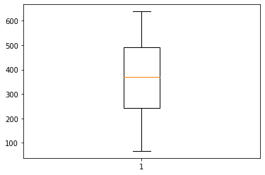
Conclusion: combining obtained statistics into a connected geo-network
import pyproj
import numpy as np
from shapely.geometry import Point
We have a set $V$ of nodes and associate geographic regions with them. Here I reduced it to some center points:
nodes = ['a', 'b', 'c']
centers = [
    Point(11.75369290168112, 48.10126143032065),
    Point(12.78652896608276, 48.70660339062048),
    Point(12.11696980992792, 49.39949287451222)
]
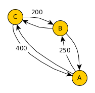
We can use above techniques to obtain distances $d_{s,t}\in\mathbb{R}$ between a source $s\in V$ and a target node $t\in V$ stored as $D = V\times V$. Given geographic points, we can also compute their geographic distance on a given projection:
wgs84_geod = pyproj.Geod(ellps='WGS84')

D = np.zeros((len(nodes), len(nodes)))
for source_idx, source_c in enumerate(centers):
    for target_idx, target_c in enumerate(centers):
        st_azimuth1, st_azimuth2, st_distance_meter = wgs84_geod.inv(source_c.x, source_c.y, target_c.x, target_c.y)
        D[source_idx][target_idx] = int(st_distance_meter/1000)
D
array([[  0., 101., 146.],
   [101.,   0.,  91.],
   [146.,  91.,   0.]])
We also know average population densities $p_{n}\in\mathbb{R}$ for each node $n\in V$:
densities = [350, 100, 500]
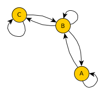
The initial structure of our geo-network can be initialized with a threshold value $\theta = 120$ (in kilometers) as $a_{s,t} = 1$ if $d_{s,t} < \theta$ or $a_{s,t} = 0$ otherwise:
A = np.where(D < 120, 1, 0)
np.array([
	[1, 1, 0],
	[1, 1, 1],
	[0, 1, 1]
])
Given the projection object, we can define a global vector as a assumption of “flow” through our geo-network. We defined this flow as the direction from Greece (EL) to Germany (DE):
global_source = nuts0_shapes[nuts0_shapes['NUTS_ID'] == 'EL'].geometry.values[0]
global_sink = nuts0_shapes[nuts0_shapes['NUTS_ID'] == 'DE'].geometry.values[0]

global_source2sink_azimuth1, global_source2sink_azimuth2, global_source2sink_dist = wgs84_geod.inv(global_source.centroid.x, global_source.centroid.y, global_sink.centroid.x, global_sink.centroid.y)
This global vector can be used to define a direction for some edges:
for source_idx, source_c in enumerate(centers):
    for target_idx, target_c in enumerate(centers):
        st_azimuth1, st_azimuth2, st_distance_meter = wgs84_geod.inv(source_c.x, source_c.y, target_c.x, target_c.y)

		# Use the azimuth as an angle to determine how far we deviate from the global vector
        if st_distance_meter > 120 and abs(st_azimuth1-global_source2sink_azimuth1) > 30:
            A[source_idx][target_idx] = 1
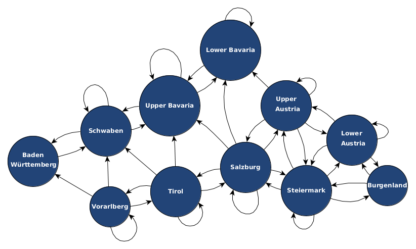
Have a look at what effect the single steps have on the geo-network:

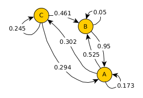
Now, given this geo-network as a basis, we can use real-world statistics and assign transition probabilities to outgoing edges for each node. Note, that as in the previous post on simulating migration flow, all edges need to add up to one to represent a valid transition probability.
A difficult question is how much of the transition probabilities to assign to the self-loop of a node. One prior assumption could be, that the higher the population density in a region is, the higher its migration pull could be. Such a prior could be implemented as defining a portion of the available transition probability from a node to be captured by this self-loop. Population densities could be as low as 354 per square kilometers in countries such as the Philippines or as high as 1,146 in Bangladesh. This prior assumption is rather naive, considering that numbers, but it shows how to approach the usage of the geo-network:
self_transition = [np.tanh(d/2000) for d in densities]
# [0.17323515783466012, 0.04995837495787998, 0.24491866240370913]
remaining = [1-np.tanh(d/2000) for d in densities]
# [0.8267648421653399, 0.95004162504212, 0.7550813375962908]
considered_distances = D*A
considered_distances
array([[  0., 101., 146.],
   [101.,   0.,   0.],
   [146.,  91.,   0.]])
Finally, we can compute a transition probability matrix for our geo-network, setting the self-loops to their population density based pulling factor and then sharing the remaining probability capacities of each node among the outgoing edges by the considered distances
T = np.zeros(A.shape)
for s_ix, source in enumerate(nodes):
    T[s_ix][s_ix] = self_transition[s_ix]

    inv_distance = [10000/considered_distances[s_ix][t_ix] if considered_distances[s_ix][t_ix] > 0 else 0.001 for t_ix, t in enumerate(nodes) if t_ix != s_ix]
    weights = np.random.dirichlet(inv_distance)
    use_weight = 0
    for t_ix, t in enumerate(nodes):
        if t_ix != s_ix:
            T[s_ix][t_ix] = weights[use_weight]*remaining[s_ix]
            use_weight += 1
T
array([[0.17323516, 0.5248695 , 0.30189534],
   [0.95004163, 0.04995837, 0.        ],
   [0.29413148, 0.46094985, 0.24491866]])
And a last check, that all of our outgoing edges sum up as transition probabilities to one:
np.sum(T, axis=1)
array([1., 1., 1.])
References
@misc{population2017,
  title={Gridded Population of the World, Version 4 (GPWv4): Population Density, Revision 11},
  url={https://sedac.ciesin.columbia.edu/data/set/gpw-v4-population-density-rev11},
  DOI={10.7927/H49C6VHW},
  publisher={Socioeconomic Data and Applications Center},
  author={Center For International Earth Science Information Network-CIESIN-Columbia University},
  year={2017}
}
-
Open Source Routing Machine: “Modern C++ routing engine for shortest paths in road networks."
-
Nominatim “is a tool to search OSM data by name and address”
-
Shapely “is a package for manipulation and analysis of geometric objects”
-
PyProj gives API access to a “cartographic projections and coordinate transformations library”