It got so quiet at our offices over the last year that I really appreciated some discussions with colleagues the last days. With Christofer I had a long talk about geo-based graphical models which I previously tried to investigate on in context of the Human+ project but in which I both struggled from a moral perspective and the level of my understanding in stochastics & statistics at that time (and today).
Now that the global covid-19 pandemic is going on, I actually see some first applications in which I could see real-world use-cases for what we have been discussing: privacy-preserved modeling of information spreading over structured models (graphical models) over time. This is actually non-trivial in a lot of senses but with the first works on network diffusion models and the success of large neural networks I see a trend in our scientific community in which we start focussing on understanding the relationships of random variables again with at the same time trying to incorporate the success of approximate methods from neural networks.
This led us to a very nice idea of thinking about graphical models which might represent geographic regions or simply random variables with distrubtions and aggregated and errorneous information exchange.
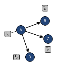
For each node $v \in {A, B, C, D}$ of our graphical model we have prior knowledge from which we can derive an estimate of how likely it is to transition to one of its target nodes.
In this graphical example we assume that there is only a transition from $A$ to either $B$, $C$ or $D$.
The number of people transitioning from $A$ to $B$ would then be represented as drawing from a multinomial distribution of which we have estimated probabilities from a dirichlet prior.
For node $A$ this would be $\alpha_0 = (10, 10, 10, 10)$ – meaning, that we are quite certain that if we transition from $A$ to any of its successor nodes either one of them is equally likely (making the multinomial distribution a discrete uniform distribution).
Drawing from $Dir(\alpha_0)$ could e.g. result in $(0.25, 0.25, 0.25, 0.25)$ and finally we come up with a draw from a multinomial distribution capturing the current information flow and the transition probability to where it goes.
$M(100, Dir(\alpha_0))$ would then give us np.random.multinomial(100, [0.25, 0.25, 0.25, 0.25]) = [31, 24, 21, 24] which we could interpret as “out of 100 people 31 stayed in $A$, 24 transitioned to $B$, 21 transitioned to $C$ and 24 transitioned to $D$”.
Given that for each time step $t_0,t_1,..$ we know how many people (up to some noise factor) are at a particular node. This observational (but privacy-preserved and errorneous) data is available as $o_0 = [100, 0, 0, 0], o_1 = [70, 20, 0, 10], o_2 = [40, 30, 10, 20]$. Now the question is: how would we update our prior knowledge $\alpha_0$?
There is an article Methods of Moments using Monte Carlo Simulation stating that for $$ \theta_{t+1} = \theta_0 + [\mu'(\theta_t)]^{-1}(\mu_0-\mu(\theta_t)) $$ with $\mu'$ being the matrix of derivatives of $\mu(\theta)$ with respect to $\theta$. Our own idea is way less formal and with theoretical background but I see quite a lot of similarities: $$ \alpha_{t+1} = \alpha_t + \gamma \frac{1}{T}\sum\limits_{t=-T}^0 p(\alpha_t)\cdot \sigma(o_t, v_t) $$ with $N$ being some rounds to sample, $p(\alpha_t)$ is a draw from the dirichlet distribution with parameters $\alpha_t$, $\sigma$ is a (somehow normalized) error signal, $o_t$ is the actual observed vector of the destination nodes and $v_t$ is the sampled (errorneous) vector of the destination nodes. I did not derive this formula so far, so there might be way more efficient sampling and update strategies out there but nevertheless it looks very similar to the optimization step in a neural network with gradient descent.
def normalize(v):
   norm = np.linalg.norm(v)
   return v/norm if norm != 0 else v
A very basic implementation could look like:
p_0 = np.array([10, 10, 10, 10])  # model parameters/prior knowledge
v_1 = np.random.multinomial(100, np.random.dirichlet(p_0))  # inference
# We just inferred [37, 17, 18, 28] as v_1 from our "model"
# normalize(o_1-v_1) gives us [ 0.78975397,  0.07179582, -0.4307749 , -0.4307749 ]
Now we could do a “naive” update step:
error = normalize(o_1-v_1)
np.maximum(np.zeros(len(p_0)), p_0+error)
# giving us p_1 = [10.78975397, 10.07179582,  9.5692251 ,  9.5692251 ]