Goal: step by step build a model to classify text documents from newsgroups20 into their according categories.

You can download the accompanying jupyter notebook for this exercise from here and use the attached environment.yml to reproduce the used conda environment..

In this exercise we want to get to know a first classifier which is commonly referred to as “naive bayes”. But don’t get discouraged by the word “naive” as it refers to the circumstance that it uses some unrealistic but practical assumptions.

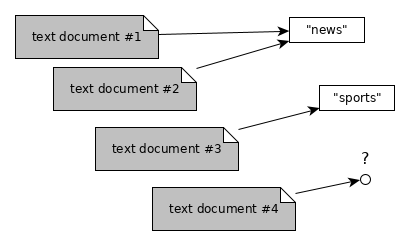
As the name suggests, in the Naive Bayes Classifier (NB) we make use of Bayes’ theorem to build a classifier. We are going to use the NB to map text documents to class labels $c \in \mathcal{C} = \{1, 2, \dots, M\}$. You could think of the example of “spam classification” from previous exercises in which we thought about a system which takes text of a mail and automatically tells whether it is spam (class “1”) or not spam (class “0”). Here, we look at a larger space of class labels ($M > 2$) and thus we’re looking at a multinomial case. In particular, we want to look at a dataset called “newsgroups20” with 20 possible classes.

Newsgroups20 can be found at http://qwone.com/~jason/20Newsgroups/ and is a popular entry classification problem in the text domain (the research field can be put into natural language processing). It contains roughly 20,000 documents from newsgroups evenly partitioned over 20 types of newsgroups. You can download the dataset on your system in your local notebook path by executing the following:

# shell scripts for downloading the data and placing it in a corresponding directory
!mkdir newsgroups
!curl -o newsgroups/news.tar.gz "http://qwone.com/~jason/20Newsgroups/20news-bydate.tar.gz"
# extract the files
!gzip -d < newsgroups/news.tar.gz | tar xf - --directory newsgroups

  % Total    % Received % Xferd  Average Speed   Time    Time     Time  Current
                                 Dload  Upload   Total   Spent    Left  Speed
100 13.7M  100 13.7M    0     0  2948k      0  0:00:04  0:00:04 --:--:-- 3400k

Let’s have a look into what we’ve downloaded: we have a directory with two sub-directories “20news-bydate-test” and “20news-bydate-train”. Both contain for each newsgroup (or class) another subdirectory. So let’s first have a look into how they are named and if there are actual 20 of them:

# Reference the paths to our dataset
base_path_newsgroups = "./newsgroups/"
path_newsgroups_train = os.path.join(base_path_newsgroups, "20news-bydate-train")
path_newsgroups_test = os.path.join(base_path_newsgroups, "20news-bydate-test")

subdirectory_names = [file_name for file_name in os.listdir(path_newsgroups_train)]
print("We have <%s> categories/subdirs in our training folder" % len(subdirectory_names))
print("Named categories:")
print("\t- "+",\n\t- ".join(sorted(subdirectory_names)))

We have <20> categories/subdirs in our training folder
Named categories:
    - alt.atheism,
    - comp.graphics,
    - comp.os.ms-windows.misc,
    - comp.sys.ibm.pc.hardware,
    - comp.sys.mac.hardware,
    - comp.windows.x,
    - misc.forsale,
    - rec.autos,
    - rec.motorcycles,
    - rec.sport.baseball,
    - rec.sport.hockey,
    - sci.crypt,
    - sci.electronics,
    - sci.med,
    - sci.space,
    - soc.religion.christian,
    - talk.politics.guns,
    - talk.politics.mideast,
    - talk.politics.misc,
    - talk.religion.misc

Understanding what the output of a classifier (a class label) looks like is now quite simple: the classifier is a function returning us one of the 20 possible class labels. How we represent a particular class is sometimes different depending on what kind of classifier we look at. We already got to learn about the trivial and the random classifier. So let’s first count how many examplary documents we have available per class / category (btw those terms are often used interchangably).

categories = sorted(subdirectory_names)
row_format ="{:>5}" * (len(categories)+1)
print(row_format.format("Cat", *range(len(categories))))
samples_per_cat = [len(list(os.listdir(os.path.join(path_newsgroups_train, cat_name)))) for cat_name in categories]
print(row_format.format("#", *samples_per_cat))

  Cat    0    1    2    3    4    5    6    7    8    9   10   11   12   13   14   15   16   17   18   19
    #  480  584  591  590  578  593  585  594  598  597  600  595  591  594  593  599  546  564  465  377

Now we create a custom “document” and we will use that document and pass it to 1) a trivial classifier, 2) a random classifier and later 3) to our naive bayes classifier.

sample_document = "some document content"

We can now “build” our trivial classifier (as a callable function). It just returns the class with the most occurences (have a look at above categories and notice, that the eleventh category “rec.sport.hockey” contains most examples).

trivial_classifier = lambda document = None: np.argmax(samples_per_cat)
trivial_classifier(sample_document)

10

categories[trivial_classifier(sample_document)]

'rec.sport.hockey'

And similar to that we “build” a random classifier. Both of them are ignorant to the actual input:

total_samples = sum(samples_per_cat)
row_format ="{:>5}" * (len(categories)+1)
print(row_format.format("Cat", *range(len(categories))))
frequency_per_category = [samples_per_cat[cat]/total_samples for cat in range(len(categories))]
print(row_format.format("Frq", *[np.round(f, 2) for f in frequency_per_category]))

  Cat    0    1    2    3    4    5    6    7    8    9   10   11   12   13   14   15   16   17   18   19
  Frq 0.04 0.05 0.05 0.05 0.05 0.05 0.05 0.05 0.05 0.05 0.05 0.05 0.05 0.05 0.05 0.05 0.05 0.05 0.04 0.03

total_samples

11314

random_classifier = lambda document = None: np.argmax(np.random.multinomial(1, frequency_per_category))
random_classifier(sample_document)

1

You could now evaluate your classifier in terms of class-wise precision, recall and calculate their macro- and micro-averaged aggregations as an exercise. In case of the random classifier, you need to once run it over all documents of the test set and then evaluate the generated assignments.

The output of a classifier could also be represented slightly different as a “one-hot”-encoding. This is often quite suitable as we can better continue further calculations with it. Also, it has a nice probabilistic interpretation in our next section.

def one_hot(cat, num_cat):
    assert cat <= num_cat
    rep = np.zeros(num_cat)
    rep[cat] = 1
    return rep

print(one_hot(trivial_classifier(sample_document), len(categories)))
print(one_hot(random_classifier(sample_document), len(categories)))

[0. 0. 0. 0. 0. 0. 0. 0. 0. 0. 1. 0. 0. 0. 0. 0. 0. 0. 0. 0.]
[0. 0. 1. 0. 0. 0. 0. 0. 0. 0. 0. 0. 0. 0. 0. 0. 0. 0. 0. 0.]

trivial_classifier(sample_document)

10

But to get to Naive Bayes we now need to clarify how we represent the input to our classifier. Currently it is a string but we need to “learn” and “calculate” something based on this input. Using a “one-hot”-encoding is the simplest approach applied to that issue of getting a numeric representation of our input: we can represent each possible word (term) as a dimension (or category) and then represent a word as one-hot-encoded vector or a document as a matrix of such vectors (or as the sum of its one-hot-terms). Example: if we only consider the words “apple”, “peach” and “orange” then we can represent the first as $(1, 0, 0)$, the second as $(0, 1, 0)$ and the third one as $(0, 0, 1)$. A document containing “apple” and “orange” could then be a matrix of two rows with those vectors $\begin{pmatrix}1 & 0 & 0\\0 & 0 & 1\end{pmatrix}$ but there are also other representations possible.

Naive Bayes

Each text document is represented as a “bag of words” - a feature vector $\mathbf{x} = (x_1, \dots, x_p)$ that has as many entries as there are words in our vocabulary $\mathcal{V}$, p = $|\mathcal{V}|$. Each dimension $i$ in $\mathbf{x}$ is associated with one word in the vocabulary. A value $x_i = 1$ if the word associated with dimension $i$ occurs in the document, and $x_i = 0$ if the word does not occur in the document.

Always keep some simple examples in mind: we can have $V = \{“apple”, “peache”, “orange”\}$ with $|V| = 3$ and we get $\mathbf{x} = (1, 0, 1)$ for a document containing “apple” and “orange”.

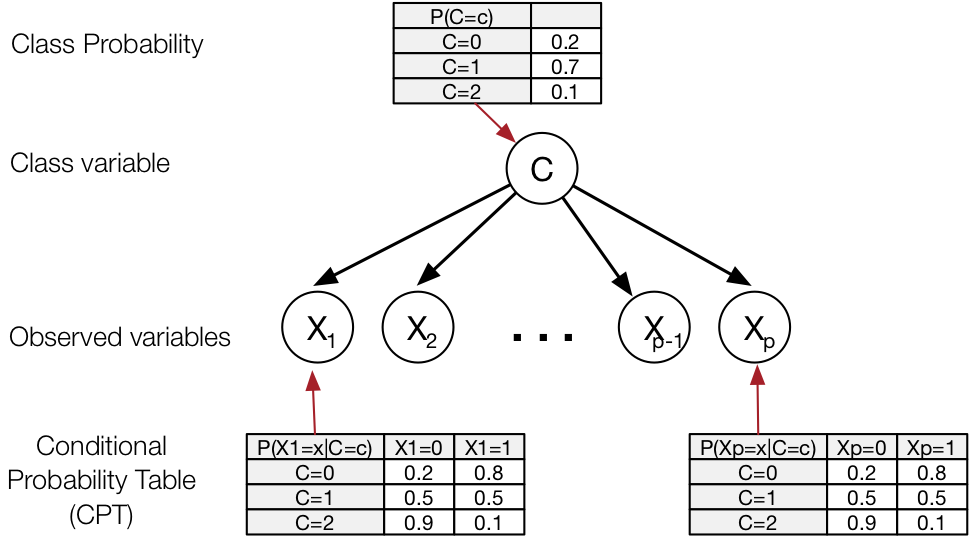
Before we can define the probabilistic model, we define the following random variables:

• $X_1, \dots, X_p$: the $p$ binary indicator random variables associated with attributes/words
• $C \in \{1, 2, \dots, M\}$: the random variable associated with the category of the document / class of the document

Given a dataset of text documents and class labels, our goal is to estimate:

$$P[C | X_1, \dots, X_p]$$

Then we can classify documents by simply finding the class $c$ that maximizes this conditional probability:

$$h(\mathbf{x}) = \argmax_{c \in \{1, 2, \dots, M\}} P[C=c | X_1=x_1, \dots, X_p=x_p]$$

We can’t estimate this quantity directly from our dataset, but by using Bayes theorem we can write:

$$P[C | X_1, \dots, X_p] = \frac{P[X_1, \dots, X_p | C] \cdot P[C]}{P[X_1, \dots, X_p]}$$

That’s already helpful. We can estimate $P[C]$ by calculating the relative frequencies of classes over all documents (regardless of their content). Remember, we already did this above: for the first category “alt.atheism” we get:

frequency_per_category[0]

0.04242531377054976

However, the joint distribution $P[X_1, \dots, X_p | C]$ is a little annoying. Even for tiny vocabulary sizes (p $\approx 100$) we would have to store and estimate $2^{100}$-1 parameters.
The Naive Bayes Classifier is called “Naive” because it makes one very strong assumption about the observation variables $X_1, \dots, X_p$: All $X_i$ are conditionally independent given the class $C$:

$$P[X_1, \dots, X_p | C] \cdot P[C] = P[C] \cdot \prod_{i=1}^p P[X_i | C]$$

Now the calculations are straight-forward. The terms $P[X_i | C]$ can be estimated by calculating the relative frequency of word $i$ per class $c$, resulting in a table of $p \cdot M$ conditional probabilities. And finally, we can make predictions by calculating:

$$h(\mathbf{x}) = \argmax_{c \in \{1, 2, \dots, M\}} P[C] \cdot \prod_{i=1}^p P[X_i | C]$$

Naive Bayes Pseudocode

Now we want to implement Naive Bayes and learn how to translate parts of the mathematical expressions into computational estimates of e.g. $P[C]$ or $P[X_i|C]$.

TrainMultiNomialNB($\mathbb C$,$\mathbb D$)

$V \leftarrow extractVocabulary(\mathbb D)$
$N \leftarrow countDocs(\mathbb D)$
for $c \in \mathbb C$:
    $N_c \leftarrow countDocsInClass(\mathbb D, c)$
    $prior[c] \leftarrow \frac{N_c}{N}$
    $text_c \leftarrow concatenateTextOfAllDocsInClass(\mathbb D, c)$
    for $t \in V$:
        $T_{ct} \leftarrow countTokensOfTerm(text_c,t)$
    for $t \in V$:
        $condprob[c][t] \leftarrow \frac{T_{ct} + 1}{\sum_{t’}(T_{ct’} + 1)}$
return $V,prior,condprob$

ApplyMultinomialNB($\mathbb C,V,prior,condprob,d$)

$W \leftarrow extractTokensFromDoc(V,d)$
for $c \in \mathbb C$:
    $score[c] \leftarrow log(prior[c])$
    for $t \in W$:
        $score[c] += log(condprob[c][t])$
return $argmax_{c \in \mathbb C} score[c]$

Implementing Multinomial Naive Bayes

What we’re now going to do is to fill below class template. We’re going to use a class as an instantiated object of it will first be “trained” on a given dataset (the newsgroups20). During this process we obtain for example how many categories we need and how large $p$ (the number of terms) is. At the end we will have a function (method of the object) which will return a class-prediction for a given document.

class NaiveBayesClassifier:
    def train(self, path):
        pass  # This has to be implemented

    def test(self, path):
        pass  # This has to be implemented
    
    def predict(self, document):
        pass  # This has to be implemented

Let’s first read a single sample of one category of our newsgroups training corpus:

exemplary_category = "comp.graphics"
examplary_category_doc = "37915"
exemplary_path = os.path.join(path_newsgroups_train, exemplary_category, examplary_category_doc)
exemplary_path

'./newsgroups/20news-bydate-train/comp.graphics/37915'

with codecs.open(exemplary_path, encoding='latin1') as file:
    pprint.pprint(file.readlines()[:40])

['From: kph2q@onyx.cs.Virginia.EDU (Kenneth Hinckley)\n',
 'Subject:   VOICE INPUT -- vendor information needed\n',
 'Reply-To: kph2q@onyx.cs.Virginia.EDU (Kenneth Hinckley)\n',
 'Organization: University of Virginia\n',
 'Lines: 27\n',
 '\n',
 '\n',
 'Hello,\n',
 '     I am looking to add voice input capability to a user interface I am\n',
 'developing on an HP730 (UNIX) workstation.  I would greatly appreciate \n',
 'information anyone would care to offer about voice input systems that are \n',
 'easily accessible from the UNIX environment. \n',
 '\n',
 '     The names or adresses of applicable vendors, as well as any \n',
 'experiences you have had with specific systems, would be very helpful.\n',
 '\n',
 '     Please respond via email; I will post a summary if there is \n',
 'sufficient interest.\n',
 '\n',
 '\n',
 'Thanks,\n',
 'Ken\n',
 '\n',
 '\n',
 "P.S.  I have found several impressive systems for IBM PC's, but I would \n",
 'like to avoid the hassle of purchasing and maintaining a separate PC if \n',
 'at all possible.\n',
 '\n',
 '-------------------------------------------------------------------------------\n',
 'Ken Hinckley (kph2q@virginia.edu)\n',
 'University of Virginia \n',
 'Neurosurgical Visualization Laboratory\n',
 '-------------------------------------------------------------------------------\n']

def tokenize_str(doc):
    return re.findall(r'\b\w\w+\b', doc) # return all words with #characters > 1

tokenize_str("I constructed this example.")

['constructed', 'this', 'example']

def tokenize_file(doc_file):
    with codecs.open(doc_file, encoding='latin1') as doc:
        doc = doc.read().lower()
        _header, _blankline, body = doc.partition('\n\n')
        return tokenize_str(body) # return all words with #characters > 1

print(tokenize_file(exemplary_path)[:10])

['hello', 'am', 'looking', 'to', 'add', 'voice', 'input', 'capability', 'to', 'user']

Iterating over the training set to “build the vocabulary”

We need to iterate over our whole dataset and read it into memory in a way that we can use its information later to compute conditional probabilities. Let’s have a first look over this loop: we are iterating over all categories (outer loop) and all documents of each category (inner loop). As a neat trick to look into these dynamics, we add zip(a_list, range(5)) to iterate only over the first five categories and within each category over the first five documents and see how many terms are in there:

for class_name, _class_idx in zip(os.listdir(path_newsgroups_train), range(5)):
    print(class_name)
    path_class = os.path.join(path_newsgroups_train, class_name)
    for doc_name, _idx in zip(os.listdir(path_class), range(3)):
        terms = tokenize_file(os.path.join(path_class, doc_name))
        print("\tdoc<%s> #terms=%s, First five terms:" % (doc_name, len(terms)), terms[:5])

comp.sys.ibm.pc.hardware
    doc<60529> #terms=118, First five terms: ['in', 'article', '1993apr19', '132748', '18044']
    doc<60402> #terms=105, First five terms: ['okay', 'here', 'is', 'my', 'configuration']
    doc<60421> #terms=48, First five terms: ['have', '486', 'machine', 'with', 'drive']
rec.autos
    doc<103011> #terms=96, First five terms: ['monthly', 'posting', 'regarding', 'the', 'buick']
    doc<102874> #terms=189, First five terms: ['in', 'article', 'c5jnk3', 'jkt', 'news']
    doc<103406> #terms=36, First five terms: ['in', 'article', 'apr16', '215151', '28035']
comp.windows.x
    doc<67169> #terms=128, First five terms: ['usually', 'when', 'start', 'up', 'an']
    doc<67113> #terms=285, First five terms: ['the', 'multi', 'lingual', 'archives', 'at']
    doc<66416> #terms=133, First five terms: ['does', 'anyone', 'have', 'any', 'good']
sci.space
    doc<61050> #terms=357, First five terms: ['in', 'article', '1993apr21', '212202', 'aurora']
    doc<61236> #terms=70, First five terms: ['can', 'tell', 'you', 'that', 'when']
    doc<61055> #terms=99, First five terms: ['related', 'question', 'which', 'haven', 'given']
talk.politics.misc
    doc<178364> #terms=244, First five terms: ['in', 'article', '1993apr17', '111713', '4063']
    doc<178413> #terms=355, First five terms: ['in', 'article', '16apr199317110543', 'rigel', 'tamu']
    doc<178587> #terms=554, First five terms: ['in', 'article', '1993apr15', '170731', '8797']

Now let’s collect that information into a pythonic structure in which we have direct access to

• a vocabulary which contains each term such as {“hello”: 2, “world”: 3}
• the size of the vocabulary
• the number of total documents
• the number of documents per category
• the number of total terms per category
• the terms within each category (after looking into all its documents)

min_count = 1
vocabulary = {}
num_docs = 0
classes = {}
priors = {}
conditionals = {}

num_docs = 0
for class_name in os.listdir(path_newsgroups_train):
    classes[class_name] = {"doc_counts": 0, "term_counts": 0, "terms": {}}
    print(class_name)
    path_class = os.path.join(path_newsgroups_train, class_name)
    for doc_name in os.listdir(path_class):
        terms = tokenize_file(os.path.join(path_class, doc_name))

        num_docs += 1
        classes[class_name]["doc_counts"] += 1

        # build vocabulary and count terms
        for term in terms:
            classes[class_name]["term_counts"] += 1
            if not term in vocabulary:
                vocabulary[term] = 1
                classes[class_name]["terms"][term] = 1
            else:
                vocabulary[term] += 1
                if not term in classes[class_name]["terms"]:
                    classes[class_name]["terms"][term] = 1
                else:
                    classes[class_name]["terms"][term] += 1

# remove terms with frequency < min_count
vocabulary = {k:v for k,v in vocabulary.items() if v > min_count}

print("Term counts per class:")
print({name: classes[name]["term_counts"] for name in classes})
print("Vocabulary size:", len(vocabulary))

comp.sys.ibm.pc.hardware
rec.autos
comp.windows.x
sci.space
talk.politics.misc
alt.atheism
sci.med
sci.crypt
rec.motorcycles
rec.sport.hockey
rec.sport.baseball
misc.forsale
comp.os.ms-windows.misc
comp.graphics
comp.sys.mac.hardware
talk.politics.guns
talk.politics.mideast
talk.religion.misc
sci.electronics
soc.religion.christian
Term counts per class:
{'comp.sys.ibm.pc.hardware': 104937, 'rec.autos': 118241, 'comp.windows.x': 159094, 'sci.space': 161284, 'talk.politics.misc': 190031, 'alt.atheism': 150831, 'sci.med': 160614, 'sci.crypt': 208234, 'rec.motorcycles': 107499, 'rec.sport.hockey': 157104, 'rec.sport.baseball': 115492, 'misc.forsale': 68699, 'comp.os.ms-windows.misc': 264777, 'comp.graphics': 116182, 'comp.sys.mac.hardware': 90823, 'talk.politics.guns': 185157, 'talk.politics.mideast': 260529, 'talk.religion.misc': 121243, 'sci.electronics': 107404, 'soc.religion.christian': 205727}
Vocabulary size: 60738

Calculating the prior probabilities and the conditional probabilities for each term

To now come up with the prior probability of the category $P(C)$ and the conditional probabilities $P(X_i|C)$ we estimate the first one simply by taking its relative document frequency. However, we apply a neat trick by working in logarithmic space (this is why in probability theory and machine learning you will often see the term log-probability (or logprob)). This costs us additional effort when computing the prior and conditional probabilities in our training phase but later we only have to sum them up - which is equivalent to multiplying them: $log(P(X_1|C))+log(P(X_2|C)) = log(P(X_1|C)*P(X_2|C))$

categories[0], classes[categories[0]]["doc_counts"]

('alt.atheism', 480)

num_docs

11314

$P(C=0)$

classes[categories[0]]["doc_counts"]/num_docs

0.04242531377054976

$log(A/B) = log(A)-log(B)$

math.log(classes[categories[0]]["doc_counts"])-math.log(num_docs)

6.173786103901937

math.log(1/len(vocabulary.values()))+math.log(5/len(vocabulary.values()))

-20.419211709219514

See how for this exemplary category we can calculate the prior $P(C)$ in “normal” space and in log space:

classes[categories[0]]["doc_counts"]/num_docs, math.log(classes[categories[0]]['doc_counts']) - math.log(num_docs)

(0.04242531377054976, -3.160010072001165)

len(vocabulary.values())

60738

categories[0]

'alt.atheism'

list(classes[categories[0]]['terms'].keys())[8], list(classes[categories[0]]['terms'].values())[8]

('chimps', 15)

sum(classes[categories[0]]['terms'].values())

150831

Now our training phase consists in calculating this prior probability for all categories and then calculate the conditionals by counting all unique terms in all documents of the particular category. Note, that we apply another technique here: laplacian smoothing by assuming that each term occurs once by default. What would happen if we would not apply it?

We could possibly have no occurences of a term within a document and therefore we would divide by zero or try to evaluate the logarithm of zero.

logspace_num_docs = math.log(num_docs)
for cn in classes:
    # calculate priors: doc frequency
    priors[cn] = math.log(classes[cn]['doc_counts']) - logspace_num_docs

    # calculate conditionals
    conditionals[cn] = {}
    cdict = classes[cn]['terms']
    terms_in_class = sum(cdict.values())

    for term in vocabulary:
        t_ct = 1.  # We assume each term to occur in each document at least once - smoothing!
        t_ct += cdict[term] if term in cdict else 0.
        conditionals[cn][term] = math.log(t_ct) - math.log(terms_in_class + len(vocabulary))

print(math.e**conditionals[categories[0]]["disturbing"], math.e**conditionals["sci.crypt"]["disturbing"])
print(conditionals[categories[0]]["disturbing"], conditionals["sci.crypt"]["disturbing"])

3.62350349305737e-06 3.599506867559147e-05
-12.52806918439661 -10.232128610124521

Calculating a score based on the conditional probabilities

print("Testing <%s>" % exemplary_path)
token_list = tokenize_file(exemplary_path)
token_list[:5]

Testing <./newsgroups/20news-bydate-train/comp.graphics/37915>





['hello', 'am', 'looking', 'to', 'add']

conditionals[categories[0]]['hello']

-11.163694176730045

np.array(frequency_per_category)

array([0.04242531, 0.05161747, 0.05223617, 0.05214778, 0.05108715,
       0.05241294, 0.05170585, 0.05250133, 0.05285487, 0.05276648,
       0.05303164, 0.05258971, 0.05223617, 0.05250133, 0.05241294,
       0.05294326, 0.04825879, 0.04984974, 0.04109952, 0.03332155])

np.array([priors[p] for p in priors])

array([-2.95367364, -2.94691686, -2.94860178, -2.94860178, -3.19175877,
       -3.16001007, -2.94691686, -2.94523477, -2.94020542, -2.93686652,
       -2.94187906, -2.96218433, -2.95198016, -2.96389519, -2.97422231,
       -3.0311772 , -2.99874192, -3.40155099, -2.95198016, -2.93853458])

scores = {}
for class_num, class_name in enumerate(classes):
    scores[class_name] = priors[class_name]
    for term in token_list: # ['hello', 'am', 'looking', ..]
        if term in vocabulary: # ['hello', 'am', ..]
            scores[class_name] += conditionals[class_name][term]
print(scores)
print("Result:")
print(max(scores, key=scores.get))

{'comp.sys.ibm.pc.hardware': -833.0541069962882, 'rec.autos': -862.3330497046505, 'comp.windows.x': -817.2169384851644, 'sci.space': -849.5240956512641, 'talk.politics.misc': -871.7723219710546, 'alt.atheism': -882.9604871670316, 'sci.med': -843.1841184508672, 'sci.crypt': -835.3925630963009, 'rec.motorcycles': -877.4131260209258, 'rec.sport.hockey': -922.3793867458648, 'rec.sport.baseball': -902.1850471341099, 'misc.forsale': -874.320329015849, 'comp.os.ms-windows.misc': -915.1018517113815, 'comp.graphics': -810.6187571263675, 'comp.sys.mac.hardware': -843.6084671998246, 'talk.politics.guns': -889.6462333560933, 'talk.politics.mideast': -899.2959096703631, 'talk.religion.misc': -893.1896022184637, 'sci.electronics': -835.1713581601585, 'soc.religion.christian': -879.8719468915807}
Result:
comp.graphics

Putting it all together

class NaiveBayesClassifier:
    def __init__(self, min_count=1):
        self._min_count = min_count
        self._vocabulary = {}
        self._num_docs = 0
        self._classes = {}
        self._priors = {}
        self._conditionals = {}
    
    def _build_vocab(self, path_base):
        self._num_docs = 0
        for class_name in os.listdir(path_base):
            self._classes[class_name] = {"doc_counts": 0, "term_counts": 0, "terms": {}}
            print(class_name)
            path_class = os.path.join(path_base, class_name)
            for doc_name in os.listdir(path_class):
                terms = tokenize_file(os.path.join(path_class, doc_name))

                self._num_docs += 1
                self._classes[class_name]["doc_counts"] += 1

                # build vocabulary and count terms
                for term in terms:
                    self._classes[class_name]["term_counts"] += 1
                    if not term in self._vocabulary:
                        self._vocabulary[term] = 1
                        self._classes[class_name]["terms"][term] = 1
                    else:
                        self._vocabulary[term] += 1
                        if not term in self._classes[class_name]["terms"]:
                            self._classes[class_name]["terms"][term] = 1
                        else:
                            self._classes[class_name]["terms"][term] += 1
        # remove terms with frequency < min_count
        self._vocabulary = {k:v for k,v in self._vocabulary.items() if v > self._min_count}

    
    def train(self, path):
        self._build_vocab(path)

        logspace_num_docs = math.log(self._num_docs)
        for cn in self._classes:
            # calculate priors: doc frequency
            self._priors[cn] = math.log(self._classes[cn]['doc_counts']) - logspace_num_docs

            # calculate conditionals
            self._conditionals[cn] = {}
            cdict = self._classes[cn]['terms']
            terms_in_class = sum(cdict.values())

            for term in self._vocabulary:
                t_ct = 1.  # We assume each term to occur in each document at least once - smoothing!
                t_ct += cdict[term] if term in cdict else 0.
                self._conditionals[cn][term] = math.log(t_ct) - math.log(terms_in_class + len(self._vocabulary))

    def test(self, path_test):
        true_y = []
        pred_y = []

        for c in self._classes:
            print(c)
            for f in os.listdir(os.path.join(path_test, c)):
                doc_path = os.path.join(path_test, c, f)
                _, result_class = self.predict_path(doc_path)
                pred_y.append(result_class)
                true_y.append(c)
        return true_y, pred_y
    
    def predict_path(self, path: str):
        token_list = tokenize_file(path)
        return self._predict(token_list)
    
    def predict(self, document: str):
        token_list = tokenize_str(document)
        return self._predict(token_list)
    
    def _predict(self, token_list: list):
        scores = {}
        for c in self._classes:
            scores[c] = self._priors[c]
            for term in token_list:
                if term in self._vocabulary:
                    scores[c] += self._conditionals[c][term]
        return scores, max(scores, key=scores.get)

clf_naivebayes = NaiveBayesClassifier()
clf_naivebayes.train(path_newsgroups_train)

comp.sys.ibm.pc.hardware
rec.autos
comp.windows.x
sci.space
talk.politics.misc
alt.atheism
sci.med
sci.crypt
rec.motorcycles
rec.sport.hockey
rec.sport.baseball
misc.forsale
comp.os.ms-windows.misc
comp.graphics
comp.sys.mac.hardware
talk.politics.guns
talk.politics.mideast
talk.religion.misc
sci.electronics
soc.religion.christian

ty, py = clf_naivebayes.test(path_newsgroups_test)

comp.sys.ibm.pc.hardware
rec.autos
comp.windows.x
sci.space
talk.politics.misc
alt.atheism
sci.med
sci.crypt
rec.motorcycles
rec.sport.hockey
rec.sport.baseball
misc.forsale
comp.os.ms-windows.misc
comp.graphics
comp.sys.mac.hardware
talk.politics.guns
talk.politics.mideast
talk.religion.misc
sci.electronics
soc.religion.christian

from sklearn import metrics

print('Accuracy: %2.2f %%' % (100. * metrics.accuracy_score(ty, py)))

Accuracy: 75.73 %

Other utility functions

#
# Code from https://scikit-learn.org/stable/auto_examples/model_selection/plot_confusion_matrix.html#sphx-glr-auto-examples-model-selection-plot-confusion-matrix-py
#

def plot_confusion_matrix(cm, classes,
                          normalize=False,
                          title='Confusion matrix',
                          cmap=plt.cm.Blues):
    """
    This function prints and plots the confusion matrix.
    Normalization can be applied by setting `normalize=True`.
    """
    if normalize:
        cm = cm.astype('float') / cm.sum(axis=1)[:, np.newaxis]
        print("Normalized confusion matrix")
    else:
        print('Confusion matrix, without normalization')

    #print(cm)

    plt.imshow(cm, interpolation='nearest', cmap=cmap)
    plt.title(title)
    plt.colorbar()
    tick_marks = np.arange(len(classes))
    plt.xticks(tick_marks, classes, rotation=90)
    plt.yticks(tick_marks, classes)

    fmt = '.2f' if normalize else 'd'
    thresh = cm.max() / 2.
    for i, j in itertools.product(range(cm.shape[0]), range(cm.shape[1])):
        plt.text(j, i, format(cm[i, j], fmt),
                 horizontalalignment="center",
                 color="white" if cm[i, j] > thresh else "black")

    plt.ylabel('True label')
    plt.xlabel('Predicted label')
    plt.tight_layout()

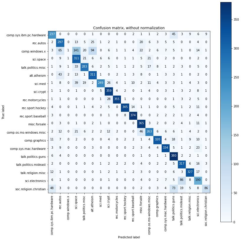
# Compute confusion matrix
cnf_matrix = metrics.confusion_matrix(ty, py)
np.set_printoptions(precision=2)

# Plot non-normalized confusion matrix
plt.figure(figsize=(12,12))
plot_confusion_matrix(cnf_matrix, classes=clf_naivebayes._classes.keys(), title='Confusion matrix, without normalization')
plt.show()

Confusion matrix, without normalization

SKlearn implementation of NaiveBayes

from sklearn.datasets import load_files
from sklearn import feature_extraction
from sklearn import metrics
from sklearn.naive_bayes import MultinomialNB

twenty_train = load_files(path_newsgroups_train, encoding='latin1')
twenty_test = load_files(path_newsgroups_test, encoding='latin1')

vectorizer = feature_extraction.text.CountVectorizer()#(max_features=len(clf.vocabulary))
train_X, train_y = vectorizer.fit_transform(twenty_train.data), twenty_train.target
test_X, test_y = vectorizer.transform(twenty_test.data), twenty_test.target
print(train_X.shape, train_y.shape, test_X.shape, test_y.shape)

(11314, 130107) (11314,) (7532, 130107) (7532,)

clf = MultinomialNB()
clf.fit(train_X, train_y)
pred_y = clf.predict(test_X)

print('Accuracy: %2.2f %%' % (100. * metrics.accuracy_score(test_y, pred_y)))

Accuracy: 77.28 %

Can we do better?

from sklearn.pipeline import Pipeline
from sklearn.feature_extraction.text import CountVectorizer
from sklearn.feature_extraction.text import TfidfTransformer
from sklearn.model_selection import GridSearchCV

# Warning: this needs some computation time!
clf = Pipeline([('vect', CountVectorizer()),
                ('tfidf', TfidfTransformer()),
                ('clf', MultinomialNB()),
               ])

parameters = {'vect__ngram_range': [(1, 1), (1, 2)],
              'tfidf__use_idf': (True, False),
              'clf__alpha': (1.0, 0.1),
             }

gs_clf = GridSearchCV(clf, parameters, n_jobs=-1)
gs_clf.fit(twenty_train.data, twenty_train.target)
pred = gs_clf.predict(twenty_test.data)

print('Accuracy: %2.2f %%' % (100. * metrics.accuracy_score(twenty_test.target, pred)))

for param_name in sorted(parameters.keys()):
    print(param_name,":", gs_clf.best_params_[param_name])

Accuracy: 81.78 %
clf__alpha : 0.1
tfidf__use_idf : True
vect__ngram_range : (1, 2)

# Warning: this needs some computation time!
from sklearn.linear_model import SGDClassifier
#SGDClassifier with hinge loss gives a linear SVM

clf = Pipeline([('vect', CountVectorizer()),
                ('tfidf', TfidfTransformer()),
                ('clf', SGDClassifier(loss='hinge', penalty='l2', alpha=1e-3, random_state=42)),
               ])

parameters = {'vect__ngram_range': [(1, 1), (1, 2)],
              'tfidf__use_idf': (True, False),
              'clf__alpha': (1e-2, 1e-3),
             }

gs_clf = GridSearchCV(clf, parameters, n_jobs=-1)
gs_clf.fit(twenty_train.data, twenty_train.target)
pred = gs_clf.predict(twenty_test.data)

print('Accuracy: %2.2f %%' % (100. * metrics.accuracy_score(twenty_test.target, pred)))

for param_name in sorted(parameters.keys()):
    print(param_name,":", gs_clf.best_params_[param_name])

Authorship

This introduction was partly created by

• Michael Granitzer (michael.granitzer@uni-passau.de)
• Johannes Jurgovsky (johannes.jurgovsky@uni-passau.de)
• Jörg Schlötterer (joerg.schloetterer@uni-passau.de)
• Julian Stier (julian.stier@uni-passau.de)

in context of the Advanced Data Science lecture at the University of Passau and with examples taken from the scikit-learn documentation.