Pruning is a surprisingly effective method to automatically come up with sparse neural networks. The motivation behind pruning is usually to 1) compress a model in its memory or energy consumption, 2) speed up its inference time or 3) find meaningful substructures to re-use or interprete them or for the first two reasons.
In this post, we will see how you can apply several quite simple but common and effective pruning techniques: random weight pruning and class-blinded, class-distributed and class-uniform magnitude-based pruning. Also, you will see how it can be very easily modularized as we do it in deepstruct. We apply a deep feed-forward neural network to the popular image classification task MNIST which sorts small images of size 28 by 28 into one of the ten possible digits displayed on them.
This post shows how to
- implement Masked Deep Feed Forward Neural Nets in PyTorch,
- how to visualize a single mask,
- what pruning is about,
- shows how to apply magnitude-based pruning, which is e.g. used in the Lottery Ticket Hypothesis (abbrev. as “IMP” = “iterative magnitude-based pruning”),
- describes pruning schemes,
- and finally lists references.
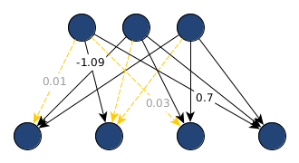
A deep feed-forward neural network nowadays simply consists of consecutive linear transformations (optionally followed by an optional layer normalization, see ba2016layer) and a non-linear activation function: $z^l = \sigma(W^lz^{l-1}+B^l)$. A three-layered network then simply looks like $y = z^3(z^2(z^1(x)))$ with $z^0 = x$ while $x$ is as usual the input and $y$ the associated target. We extend this formulation technically to explicitly apply binary masks on the weights, so we can later reset representations to initial distributions and still keeping the learned structural information. This works by adding a multiplicative binary mask matrix in the shape of the weight matrix: $z^l = \sigma((W^l\odot M^l)z^{l-1}+B^l)$ with $\odot$ being the hadamard (pointwise) product.
From a technical perspective, pruning sets values in the weight matrix $W^l$ to zero or – to keep the information about the weight in memory – sets the associated binary value in $M^l$ to zero:
$$\begin{pmatrix}0.01 & -0.4 & 1.2 \\ -1.09 & 0.35 & 0.2 \\ 0.03 & 2.3 & -1.03 \\ 0.7 & -0.45 & 0.82 \end{pmatrix} \odot \begin{pmatrix}0 & 1 & 1 \\ 1 & 0 & 0 \\ 0 & 1 & 1 \\ 1 & 1 & 1\end{pmatrix} \cdot x^v + B^v$$
with $x^v \in \mathbb{R}^3, B^v \in \mathbb{R}^4$.
Masked Deep Feed-Forward Neural Nets
The following can be skipped if you are only interested in pruning. This section shows the code for constructing arbitrarily deep feed-forward neural networks with a one-liner:
my_mnist_module = MaskedDeepFFN((1, 28, 28), 10, [100, 100, 100], use_layer_norm=True)
In PyTorch, the implementation of $(W^l\cdot M^l)x$ boils down to F.linear(x, self.weight * self.mask, self.bias) with appropriate class properties.
We are following the implementations in deepstruct, a pytorch extension, to not just add this mask matrix but also prepare for further PyTorch modules which might contain maskable elements.
class MaskedLinearLayer(torch.nn.Linear, MaskableModule):
    def __init__(self, in_feature: int, out_features: int, bias=True, keep_layer_input=False):
        """
        :param in_feature: Number of input features
        :param out_features: Output features in analogy to torch.nn.Linear
        :param bias: Iff each neuron in the layer should have a bias unit as well.
        """
        super().__init__(in_feature, out_features, bias)

        self.register_buffer('mask', torch.ones((out_features, in_feature), dtype=torch.bool))
        self.keep_layer_input = keep_layer_input
        self.layer_input = None

    def forward(self, input):
        x = input.float()  # In case we get a double-tensor passed, force it to be float for multiplications to work

        # Possibly store the layer input
        if self.keep_layer_input:
            self.layer_input = x.data

        return F.linear(x, self.weight * self.mask, self.bias)
Note, that we also added an additional parent class module called MaskableModule in case we will work with other layers that will contain binary masks:
def maskable_layers(network):
    for child in network.children():
        if type(child) is MaskedLinearLayer:
            yield child
        elif type(child) is nn.ModuleList:
            for layer in maskable_layers(child):
                yield layer

class MaskableModule(nn.Module):
    def apply_mask(self):
        for layer in maskable_layers(self):
            layer.apply_mask()

    def recompute_mask(self, theta=0.0001):
        for layer in maskable_layers(self):
            layer.recompute_mask(theta)
Now a module with multiple masked linear layers would simply repeat these MaskedLinearLayer objects. In pytorch, you can simply add them all into a torch.nn.ModuleList and the submodule object is then part of the parent module and its parameters are registered to be considered in a backward pass during learning. During the forward pass, each linear layer should be followed by a non-linear activation function such as a rectified linear unit function max(0,x). When also considering optional layer normalization modules a full implementation for a MaskedDeepFFN with multiple hidden layers can be implemented as in the following code.
class MaskedDeepFFN(MaskableModule):
    def __init__(self, size_input, size_output: int, hidden_layers : list, use_layer_norm: bool = False):
        super(MaskedDeepFFN, self).__init__()
        assert len(hidden_layers) > 0

        self._activation = torch.nn.ReLU()

        # Multiple dimensions for input size are flattened out
        if type(size_input) is tuple or type(size_input) is torch.Size:
            size_input = np.prod(size_input)
        size_input = int(size_input)

        self._layer_first = MaskedLinearLayer(size_input, hidden_layers[0])
        self._layers_hidden = torch.nn.ModuleList()
        for l, size_h in enumerate(hidden_layers[1:]):
            self._layers_hidden.append(MaskedLinearLayer(hidden_layers[l], size_h))

            if use_layer_norm:
                self._layers_hidden.append(torch.nn.LayerNorm(size_h))

            self._layers_hidden.append(self._activation)

        self._layer_out = MaskedLinearLayer(hidden_layers[-1], size_output)

    def forward(self, input):
        # input : [batch_size, ?, ?, ..], e.g. [100, 1, 28, 28] or [100, 3, 32, 32]
        out = self._activation(self._layer_first(input.flatten(start_dim=1)))  # [B, n_hidden_1]
        for layer in self._layers_hidden:
            out = layer(out)
        return self._layer_out(out)  # [B, n_out]
Note, how simple it now gets to construct such a multi-layer perceptron with masking capabilities:
my_mnist_module = MaskedDeepFFN((1, 28, 28), 10, [100, 100, 100], use_layer_norm=True)
This module now accept inputs in the shape of a MNIST dataset and the final layer maps to ten possible output neurons which are interpreted as the individual class logits of each digit to be recognized – which are then
Visualizing a single mask
A mask can be simply accessed through layer.mask and in case of our composed deep feed-forward model above the first layer can be accesses with my_mnist_module._layer_first.mask.
import seaborn as sns

# select a layer out of the model
lay = next(maskable_layers(model))
lay.recompute_mask(theta=0.04)
# get one side of the square of the feature size
side = int(np.sqrt(len(lay.weight[0])))
# plot a heatmap of the incoming connections to one particular neuron
sns.heatmap(lay.mask[0].reshape((side, side)).cpu().detach().numpy(), cmap="Blues")
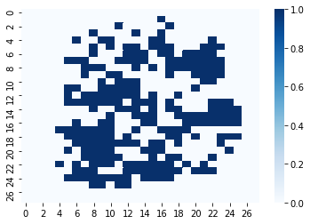
With the above implementation a mask or the weights can be easily visualized in seaborn / matplotlib. For practical purposes layer sizes are set to squares of natural numbers because all the incoming connections to a single neuron are then visualizable as a two-dimensional image. Often sizes such as $100 = 10\times 10$ or $256 = 16\times 16$ are of practical use. Note, that a threshold of $\theta = 0.04$ is used to re-compute the mask. This is a magnitude-based pruning approach in which all weights below $\theta$ are set to zero. Otherwise just a few connections would be at zero.
Also, the weight magnitude can be visualized. To have it visually appealing and recognize singularities (zero-connections) easily, we visualize the absolute value of a weight instead of the actual value - whether it is negative or positive. Values away from zero can be interpreted as “meaningful” - at least this is the assumption in magnitude-based pruning.
# plot a heatmap of the weight intensity
sns.heatmap(np.abs(lay.weight[0].reshape((side, side)).cpu().detach().numpy()))
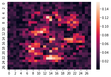
In these figures here, the mask and weights of the first layer are depicted. These refer to the feature space and we can easily see that in MNIST standard feed-forward neural networks exhibit a focus-area in the middle where the digits are usually places. MNIST is carefully constructed to have this property and we can observe that the information at the border of the image is less important to classify the digits contained in the dataset. Such an appealing interpretation is hardly obtained when looking into deeper structures, especially because the hidden feature spaces are automatically derived through backpropagation and contain compressed information.
Pruning
Pruning can be organized in two key components: first, a pruning criterion has to be chosen and second, a scheme needs to be defined. A pruning criterion assigns a rank to a set of elements to be pruned and thus puts them in order. For random pruning, this is simply a random ranking. The scheme, on the other hand, chooses how many elements are to be pruned. Further, one can apply pruning on multiple sets of elements and not just one. These multiple sets can be considered as a class among which elements are to be selected according to the criterion. In context of magnitude based pruning the definition of the element set under consideration is known to make a huge difference (see marchisio2018prunet).
Magnitude-based pruning
Magnitude-based pruning is quite related to $\mathcal{L}_1$-regularization through the objective but being applied outside the learning loop. In magnitude-based pruning weights are simply set to zero if they fall below a certain threshold $\theta$: $M_{ij} = 0$ iff $w_{ij} < \theta$. Therefore, MBP ranks weights according to the magnitude of their current value. For neurons, one could also rank them according to the sum of their weight values.
The threshold $\theta$ acts as an additional hyperparameter for the overall neural network model. In some pruning schemes (see below) this threshold can be obtained automatically based on a whole set of weights, e.g. from all neurons of one layer while in other contexts it is simply set to e.g. $\theta = 0.05$ and it can be investigated on in an ablation study.
From visuals of experiments in stier2021experiments, you can quite easily see that magnitude based pruning actually has a meaningful impact when compared to pruning elements randomly.
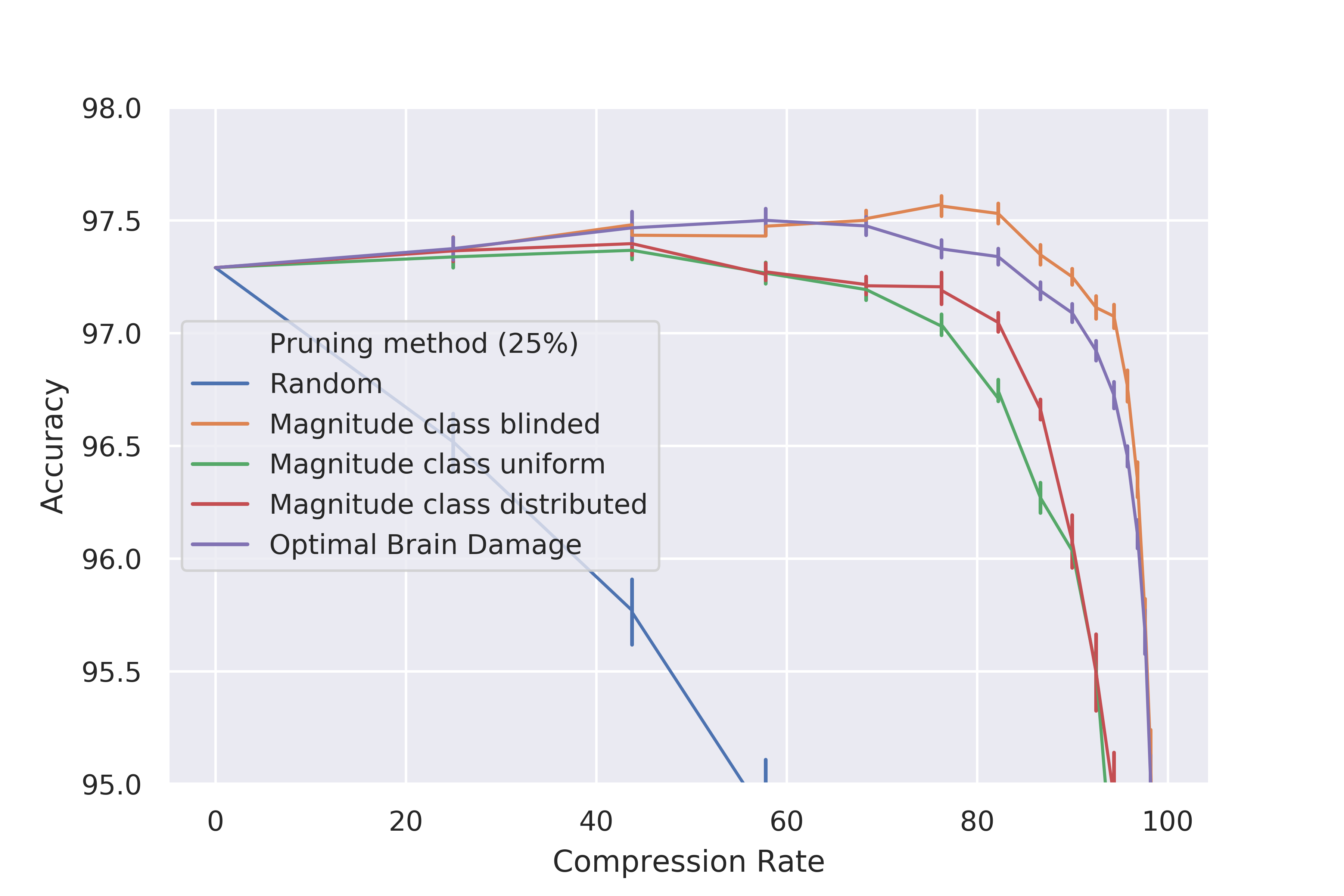
See et al. see2016compression propose three different possibilities for magnitude-based percentage pruning (called in that context schemes but I understand s.th. different about pruning schemes as seen below): a) class-blinded, b) class-uniform and c) class-distributed pruning. In class-blinded pruning, simply all weights or elements of the network are taken into consideration when sorting and selecting the top p% of them. Blinded refers to the circumstance that layers or other structuring elements are not taking into account such that some are more affected than others. In class-uniform pruning, the sorting is done within layers or other structuring elements (e.g. blocks). This leads to exactly pruning p% of each layer. In class-distributed pruning the standard deviation $\sigma_c$ of the magnitude of elements within each class are computed and after sorting the elements within each class, all elements below the threshold $\lambda\sigma_c$ are pruned.
How to apply magnitude-based pruning based on a fixed threshold $\theta$ on the absolute magnitude of the weights:
def recompute_mask(self, theta: float = 0.001):
    self.mask = torch.ones(
        self.weight.shape, dtype=torch.bool, device=self.mask.device
    )
    self.mask[torch.where(abs(self.weight) < theta)] = False
A full pipeline of model construction, training and a pruning step per each epoch can then look like the following (leaving out loading data or batching it):
import deepstruct.sparse

device = torch.device("cuda:0" if torch.cuda.is_available() else "cpu")
model = deepstruct.sparse.MaskedDeepFFN(784, 10, [1000, 500, 200, 100])
model.to(device)
loss = torch.nn.CrossEntropyLoss()
optimizer = torch.optim.Adam(model.parameters(), lr=0.01)
# Iterate several iterations over the same data
for epoch in range(100):
    # Load data from a data loader (batch-wise)
    features, labels = get_data_batch()
    # Reset cached gradients in optimizer
    optimizer.zero_grad()
    # Perform inferencing step of model to obtain guessed classes
    prediction = model(features)
    # Calculate current error for pairs of predictions and known class labels
    error = loss(prediction, labels)
    # Compute gradient through the deep learning model
    error.backward()
    # Perform update step with gradient descent
    optimizer.step()

    # Possibly conduct a pruning step
    model.recompute_mask(theta=0.01)
Pruning Schemes
Various pruning schemes can be used to investigate on or apply pruning to a neural network. A single pruning step is usually called one shot pruning. This is especially useful to compare different pruning methods to assess how much they affect the network once and can be also thought of as a measure on how much information from the networks ability is reduced. Most commonly, iterative pruning is applied in which at each step a certain number or proportion of elements are removed based on the selection method. Iterative magnitude based pruning, often abbreviated as IMP, is the most prominent and well-studied approach. Based on the selection method, one can e.g. choose the top-$k$ ($k\in\mathbb{N}$) or the top-$p$ ($p\in[0,1]$) elements to be removed per step and iterate until some stopping criterion such as a maximum number of steps, a minimum number of remaining elements or some performance measure threshold of the network after re-training is reached. Somewhat less popular is bucket-based pruning in which a bucket of some quantified measure of the elements is filled up in each step. For magnitude based pruning, a bucket could consist of the summed magnitude of all weights such that in each step up to a value of $\beta = 10$ can be pruned or for saliency-based methods a certain saliency threshold is reached.
Summary
Pruning is a very simple and often effective technique for compressing neural nets or making them at least sparse. Obtained structures can be technically imposed on the network by using binary masks, which can be later easily analyzed, visualized or re-used in other networks. Pruning provides an alternative to regularization through the optimization loss or can even be combined, although regularization only leads to sparsity under certain circumstances, e.g. using the appropriate norm and activation functions such as rectified linear units fostering real sparsity.
Sparsity could occur due to overparamterization and in the input feature space it could be due to dependencies in the data the network learns about. When sparsity occurs in the hidden layers the simplest explanation is also overparameterization. But it could also be that hidden layers exhibit structure that fosters the performance. I call this second idea the “Hidden Structural Prior Hypothesis”. To which extend sparsity and structure have an influence on deep neural networks is an ongoing debate. Understanding it might lead to improved Neural Architecture Search and eXplainable AI techniques.
References
@article{stier2021experiments,
  title={Experiments on Properties of Hidden Structures of
Sparse Neural Networks},
  author={Stier, Julian J and Darji, Harshil and Granitzer, Michael},
  journal={arXiv preprint arXiv:2107.12917},
  year={2021}
}
@article{ba2016layer,
  title={Layer normalization},
  author={Ba, Jimmy Lei and Kiros, Jamie Ryan and Hinton, Geoffrey E},
  journal={arXiv preprint arXiv:1607.06450},
  year={2016}
}
@inproceedings{han2015learning,
	title={Learning both weights and connections for efficient neural network},
	author={Han, Song and Pool, Jeff and Tran, John and Dally, William},
	booktitle={Advances in neural information processing systems},
	pages={1135--1143},
	year={2015}
}
@inproceedings{marchisio2018prunet,
	title={PruNet: Class-Blind Pruning Method for Deep Neural Networks},
	author={Marchisio, Alberto and Hanif, Muhammad Abdullah and Martina, Maurizio and Shafique, Muhammad},
	booktitle={2018 International Joint Conference on Neural Networks (IJCNN)},
	pages={1--8},
	year={2018},
	organization={IEEE}
}
@article{frankle2018lottery,
  title={The lottery ticket hypothesis: Finding sparse, trainable neural networks},
  author={Frankle, Jonathan and Carbin, Michael},
  journal={arXiv preprint arXiv:1803.03635},
  year={2018}
}
@article{see2016compression,
  title={Compression of neural machine translation models via pruning},
  author={See, Abigail and Luong, Minh-Thang and Manning, Christopher D},
  journal={arXiv preprint arXiv:1606.09274},
  year={2016}
}