From my work on generative models for graphs to learn distributions of graphs for Neural Architecture Search I started exploring graphs from an auto-regressive and an probabilistic perspective. Auto-regressive in this context means that the non-canonical representation used for a graph is based on a sequence in which the order matters and builds upon the previous step. The probabilistic perspective refers to a new idea for representing graphs not deterministically but with a representation which already supports some kind of fuzziness.
Problems with Graph Isomorphism
A graph is commonly represented visually, with an adjacency matrix or an adjancency list. The adjacency matrix and adjacency list representation have wide-spread purposes as data structures and provide very well-analysed runtimes for graph operations such as adding a vertex or removing an edge.
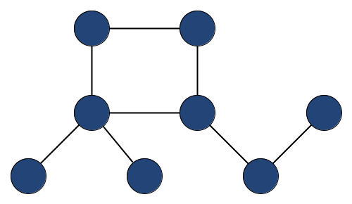
For the minimal graph example you can use python and networkx and the following code to instantiate the graph:
import matplotlib.pyplot as plt
nx.draw(G)
plt.show()
G = nx.Graph()
G.add_nodes_from(np.arange(8))
G.add_edges_from([(0,1), (1,2), (1,3), (3,4), (4,5), (3,6), (6, 7), (7,1)])
nx.draw(G)
plt.show()
We can obtain an adjacency list representation with:
list(nx.adjlist.generate_adjlist(G))
and obtain ['0 1', '1 2 3 7', '2', '3 4 6', '4 5', '5', '6 7', '7'] or we can get an adjacency matrix representation with:
nx.adjacency_matrix(G).todense()
matrix([[0, 1, 0, 0, 0, 0, 0, 0],
        [1, 0, 1, 1, 0, 0, 0, 1],
        [0, 1, 0, 0, 0, 0, 0, 0],
        [0, 1, 0, 0, 1, 0, 1, 0],
        [0, 0, 0, 1, 0, 1, 0, 0],
        [0, 0, 0, 0, 1, 0, 0, 0],
        [0, 0, 0, 1, 0, 0, 0, 1],
        [0, 1, 0, 0, 0, 0, 1, 0]], dtype=int64)
Now let’s just look at a graph, which has two more vertices added to the tail of this small chain coming out of the circle of four vertices:
G.add_nodes_from([8, 9])
G.add_edges_from([(5,8), (8,9)])
such that we obtain now the following two representations:
['0 1', '1 2 3 7', '2', '3 4 6', '4 5', '5 8', '6 7', '7', '8 9', '9']

matrix([[0, 1, 0, 0, 0, 0, 0, 0, 0, 0],
        [1, 0, 1, 1, 0, 0, 0, 1, 0, 0],
        [0, 1, 0, 0, 0, 0, 0, 0, 0, 0],
        [0, 1, 0, 0, 1, 0, 1, 0, 0, 0],
        [0, 0, 0, 1, 0, 1, 0, 0, 0, 0],
        [0, 0, 0, 0, 1, 0, 0, 0, 1, 0],
        [0, 0, 0, 1, 0, 0, 0, 1, 0, 0],
        [0, 1, 0, 0, 0, 0, 1, 0, 0, 0],
        [0, 0, 0, 0, 0, 1, 0, 0, 0, 1],
        [0, 0, 0, 0, 0, 0, 0, 0, 1, 0]], dtype=int64)
Note, that the list representation was increased with two entries with two vertices and two edges and the adjacency matrix representation increased from $8\times 8$ to $10\times 10$ in its dimensions.
In deep learning, much is about automatically learning good feature representations. The issue with graphs, however is quite present in this example: for the adjacency list representation consider the following example:
G2 = nx.relabel_nodes(G, {i: 9-i for i in G.nodes})
nx.adjacency_matrix(G2).todense()
for which we obtain ['9 8', '8 7 6 2', '7', '6 5 3', '5 4', '4 1', '3 2', '2', '1 0', '0'].
The graph G2 is obviously isomorphic to G1 as we just relabelled it.
Also, the list representation did not change in structure except for relabelling the values.
But here’s a crux:
If we use the adjacency list, the labelling values have a very important effect in this representation.
A change in a single value means that the structure can inherently change.
If we replace ‘5 8’ in G with ‘5 9’, we obtain an isomorphic graph but if we change ‘3 4 6’ to ‘3 4 5’ we break up the circle of four vertices and create a triangle at the same time with other vertices.
This is very sensitive when you compare it to images which are composed of pixel-values in a grid:
changing a value slightly only affects a very local region of the image and only changes the visual appearing with a small change in color (depending on the used color space).
If we use the adjacency matrix, the whole dimensions expand - although we could look at the smaller graph of eight vertices as being embedded in the larger graph, but then we would need to consider infinitely large matrices which gets us into total different mathematical fields and issues.
Deep Learning and Graphs
Now what’s the actual set of problems we’d like to tackle? With generative models for graphs one goal is to draw random graphs from an unknown family of graphs or a partially described distribution of graphs: $g \sim P(G)$. This notation can be seen in analogy to e.g. $n \sim \mathcal{N}(\mu=0;\sigma=1.0)$, so drawing a number from a standard gaussian distribution. How is such a $n$ obtained in practice? An example is the Box-Muller transform to transform two uniformly sampled numbers into realizations of a normally-distributed random variable – and the uniformly sampled numbers then come from the machine’s pseudorandom number generator (PRNG).
There exist majorly three types of generative models for graphs: first, the probabilistic models from network science such as Erdős-Rényi, Barabasi-Albert, Watts-Strogatz or Kleinberg. These have specific rules and only few probabilistic influences such as draws from a binomial distribution $x_i ∼ B(1,p)$ in which $x_i$ decide whether a edge is present or not. Fascinatingly, certain patterns emerge from these models and they define distinguishable families of graphs although a graph can be in multiple families with some probability – from a set theoretical perspective these models define fuzzy sets. Secondly, statistical models which allow to approximate a given graph with a resulting graph with similar properties such as when comparing its degree distribution, diameter or spectrum. An example is the KronFit algorithm. Thirdly, statistical models which allow to learn a distribution over graphs given a set of exemplary graphs $g\in \{g_1,\dots,g_d\} = D \sim P(G)^d$ - these are of high interest since the advancements of geometric deep learning and various message passing techniques. The idea is often that we have a natural process for which we can observe $D = D_{train}\cup D_{test}$ and we want to learn a model $f$ on $D_{train}$ which is able to sample similar graphs as coming from this natural process. Such models are then evaluated with comparing a generated set of graphs $\hat{D}$ with an unseen test set $D_{test}$ - due to the complexity and size of graphs this metric is often based on property distributions over all graphs or most recently on comparisons in graph manifolds.
Now, some of the recent deep learning models for generating graphs are based on an auto-regressive representation of a graph - something which was already cast in the GraphRNN (see You2018) paper. I called it later construction sequences in the context of DeepGG (see Stier2021) in which we analysed an extension and an inherent structural bias towards scale-freeness of DGMG (see Li2018).
This finally brings me to my research on what I currently call assembly representations for graphs which might not only be interesting to sample a single graph from an unknown or partially described distribution but also interesting in context of temporal or evolutionary formulations of graphs. The starting point is the idea to generalize the concept of letting a graph emerge from an initial state with successive application of operations. If we think back to the adjacency list representation we see a successive application of adding a vertex and all edges for that vertex. For the adjacency representation, we can look at it as $n$ successive vectors of size $n$ for which we define whether an edge is present or not. In both cases the order or the vertex labelling matters for the overall representation. The adjacency list representation could be even compacted to take the order of the vertices into account and by this omit the particular source vertex (however, you need empty edge lists then for unconnected vertices).
Now, given any sequence of operations we can assemble a graph by following the sequence and apply the operation on the current state of the graph – as each step depends on the previous one we obviously have an auto-regressive representation but as we now saw, we can even say that every introcued representation is in some way auto-regressive.
Why would that be of interest? The operation used for assembling the object which we observe from a natural process casts a bias on how the object is fundamentally emerging and while a deep learning model might learn representations for chemicals or molecules that way it might inherently have advantages or disadvantages (without valuing the bias). Possibly, if we now the predicates for how the chemical compound is assembled in an operational way we might have a better representation to learn about this process and might be able to improve discriminative or generative models for these compounds.
Graph Operations
Below, I collected some notation to think about such assembly representations.
One interesting part of it is to not represent the assembled objects deterministically but to already let the representation reflect fuzzy sets.
This allows for operations that are way more high-level than very specific operations and do not need too much parameterization in the sequence.
Imagine the previously used construction sequences with [ N N E 0 1 N E 0 2 ] which is a deterministic way of representing the graph $\circ~–~\circ~–~\circ$ while a twine such as [ V V E V E ] represents an isomorphic (exactly the same) graph – V and N denote adding a vertex and E adding an edge.
To know which kind of example representation we talk about, we work with these symbols N and E for the deterministic (parameterized versions) and with V and E for the more probabilistic versions for now.
Only when it gets larger, a twine starts to get fuzzy (depending on the operations), e.g. [ V V E V E E V E ] represents now two possible graphs
  ____
 /    \
o--o--o---o  ,

  ____
 /    \
o--o--o  ,
   |
   o
With this in mind, we now have a fuzzy representation for sets of graphs and one that can be really short. How short? For each graph we would like to represent we could have an own representation. Then we would encode all the information in our underlying “alphabet” - the set of operations used for the assembly. Of course, this is not of much use, as a language which has a symbol for each word is too complex. Assumably, there is a “good” tradeoff between operation set size and representative quality. If we look at the construction sequences we only have two operations and we intuitively know that each graph can be represented with this notation. Can we find other operation sets to achieve this property of universality? More generally, for a possibly infinite target set of objects (graphs), can we find a finite set of operations such that the union of all finite assembling sequences are a superset of this target set or even equivalent to it? It would be further desirable to restrict the number of operations. Two operations - adding a vertex and adding an edge - seems to be clearly a minimum, but could we further try to optimize the operation set such that the sequence lengths get minimal in some sense? Or could we even achieve that certain minimal sequence lengths have only restrictive overlaps between each other?
For the above two graphs we could have a deterministic sequence of $\{$[ N N E 0 1 N E 0 2 E 1 2 N E 2 3 ], [ N N E 0 1 N E 0 2 E 1 2 N E 1 3 ]$\}$ but we could also represent it with $\{$[ N N N N E 3 2 E 2 1 E 2 0 E 1 0 ], [ N N N N E 2 0 E 2 1 E 1 0 E 3 1 ]$\}$.
| $g$ | a single graph |
| $V_g$ | finite set of vertices of a graph $g$ with $|g| = |V_g|$ being the number of its vertices |
| $E_g \subset V_g\times V_g$ | finite set of edges for $g$ |
| $G$ | set of graphs; $G^{\geq v}$ denotes $\{g ~|~ g\in G \land |g| \geq v\} \subseteq G$ |
| $\mathcal{G}$ | the infinite set of all graphs |
| $o: \mathcal{G}\rightarrow\mathcal{G}$ | an operation (mapping) transforming a graph into another graph |
| $O$ | a (finite) set of operations |
| $[o_1, o_2, o_3]$ | "twine": a finite sequence of graph operations |
| $g[o]$ | "wad": the set of graphs resulting from all mappings when applying $o$ on an initial graph $g$; if $g$ is the empty graph we write $\circ [o]$. |
| $g [o_1, o_2, o_3]$ | the successive application of three operators of a twine on an inital graph g: $o_3(o_2(o_1(g)))$ |
| $\mathcal{S}^{O^s}$ | $ = \{[a_1, a_2, \dots, a_s] ~|~ a_i \in O, \forall i\in\{1,\dots,s\}\}$ the set of all possible sequences of length $s$ over successive applications of operations from $O$ |
| $\mathcal{S}^{O}$ | $= \bigcup_{j\in\mathbb{N}} \mathcal{S}^{O^j}$ the infinite set of all possible any-length sequences of operations $O$ |
| $G[\mathcal{S}^O]$ | $= \{ g~t ~|~ t\in\mathcal{S}^O, g\in G\}$ the infinite "wad" of an finite operation set and a set of source graphs. For a single graph we can write $g[\mathcal{S}^O]$ |
| $\mathcal{S}^O(g)$ | $= \{ t\in\mathcal{S}^O ~|~ g\in\circ~t: \}$ the set of all any-length sequences of operations $O$ which assemble $g$ |
Thoughts & Questions:
- can we divide mappings into ones that keep stable in the size of their wad, grow logarithmically or linearly with respect to the vertices or edges or super-linearly?
- is there a finite $O$ which is small (!) such that $\circ[\mathcal{S}^O] = \mathcal{G}$? (= generating set)
- is there a finite $O$ which is small (!) such that $\circ[\mathcal{S}^O] = G$? (= generating set but not universal)
- min twines: given a generating set $O$ and a graph $g$, let the minimal twines be $T^O(g) = \{ t\in\mathcal{S}^O ~|~ g\in\circ t \land \forall t_2\in\mathcal{S}^O: |t| \leq |t_2|\}$ - can $T^O(g)$ be finite and small? can $T^O(g)$ be empty? The idea of minimal twines is to have the set of minimal-length assembly description for a graph under the considered operation set.
- sharp twines: $ST^O(g) = \{t\in T^O(g) ~|~ \text{such that} ~ |\circ~t| \leq |\circ~t_2| ~ \forall t,t_2\in T^O(g) \}$. The idea of sharp (minimal) twines is to have a set of minimal-length assembly descriptions which then also are small sets of graphs to reduce fuzzyness or to measure how distinctive one reaches a particular graph.
References
@inproceedings{stier2021deepgg,
  title={DeepGG: A deep graph generator},
  author={Stier, Julian and Granitzer, Michael},
  booktitle={International Symposium on Intelligent Data Analysis},
  pages={313--324},
  year={2021},
  organization={Springer}
}
@inproceedings{you2018graphrnn,
  title={Graphrnn: Generating realistic graphs with deep auto-regressive models},
  author={You, Jiaxuan and Ying, Rex and Ren, Xiang and Hamilton, William and Leskovec, Jure},
  booktitle={International conference on machine learning},
  pages={5708--5717},
  year={2018},
  organization={PMLR}
}
@article{li2018learning,
  title={Learning deep generative models of graphs},
  author={Li, Yujia and Vinyals, Oriol and Dyer, Chris and Pascanu, Razvan and Battaglia, Peter},
  journal={arXiv preprint arXiv:1803.03324},
  year={2018}
}